
Table of Contents
Trade mis-invoicing in Africa
Policy and media attention on illicit financial flows (IFF) has increased, with the recognition that Africa is a net creditor to the world.
 |
 |
|
| New York Times (2013) | Guardian (2015) | |
 |
 | |
| Guardian (2017) | Economist (2019) |
What is trade mis-invoicing?
The deliberate mis-statement of price or quantity of internationally traded goods in invoices presented to customs
Can occur at import or export
Can result in an inflow or outflow of money
Motivations for trade mis-invoicing include:
Evading tariffs
Exploiting subsidy regimes
Subverting forex and capital controls
Hiding transfers of wealth
Mechanisms of mis-invoicing
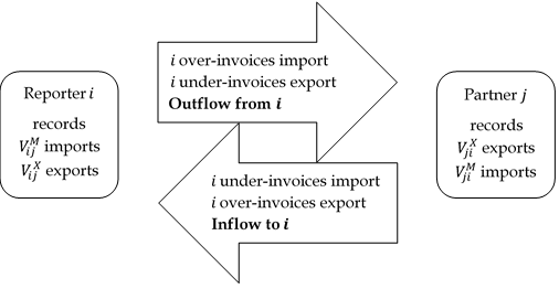
From the reporting country’s perspective, trade mis-invoicing can result in an inflow or an outflow of capital, and this can be achieved by misreporting the value of both imports and exports. Money can be moved out of the country by over-invoicing imports, where that country pays too much money to buy goods from its partner; or by under-invoicing exports, where that country does not charge enough money for the goods that it sells to its partner. Conversely, money can be illicitly routed in to that country by under-invoicing imports, where the country pays too little money to buy goods from its partner; or by over-invoicing exports, where the country charges too much for the goods that it sells to its partner. The direction of trade mis-invoicing in addition to its mechanisms is represented in the diagram below.
Why does trade mis-invoicing matter?
Outflows undermine the fiscal base and public spending
Financing gap needed to meet the Sustainable Development Goals (SDGs)
Combating trade mis-invoicing is crucial for the mobilization of domestic resources in the continent, and can catalyze sustainable development
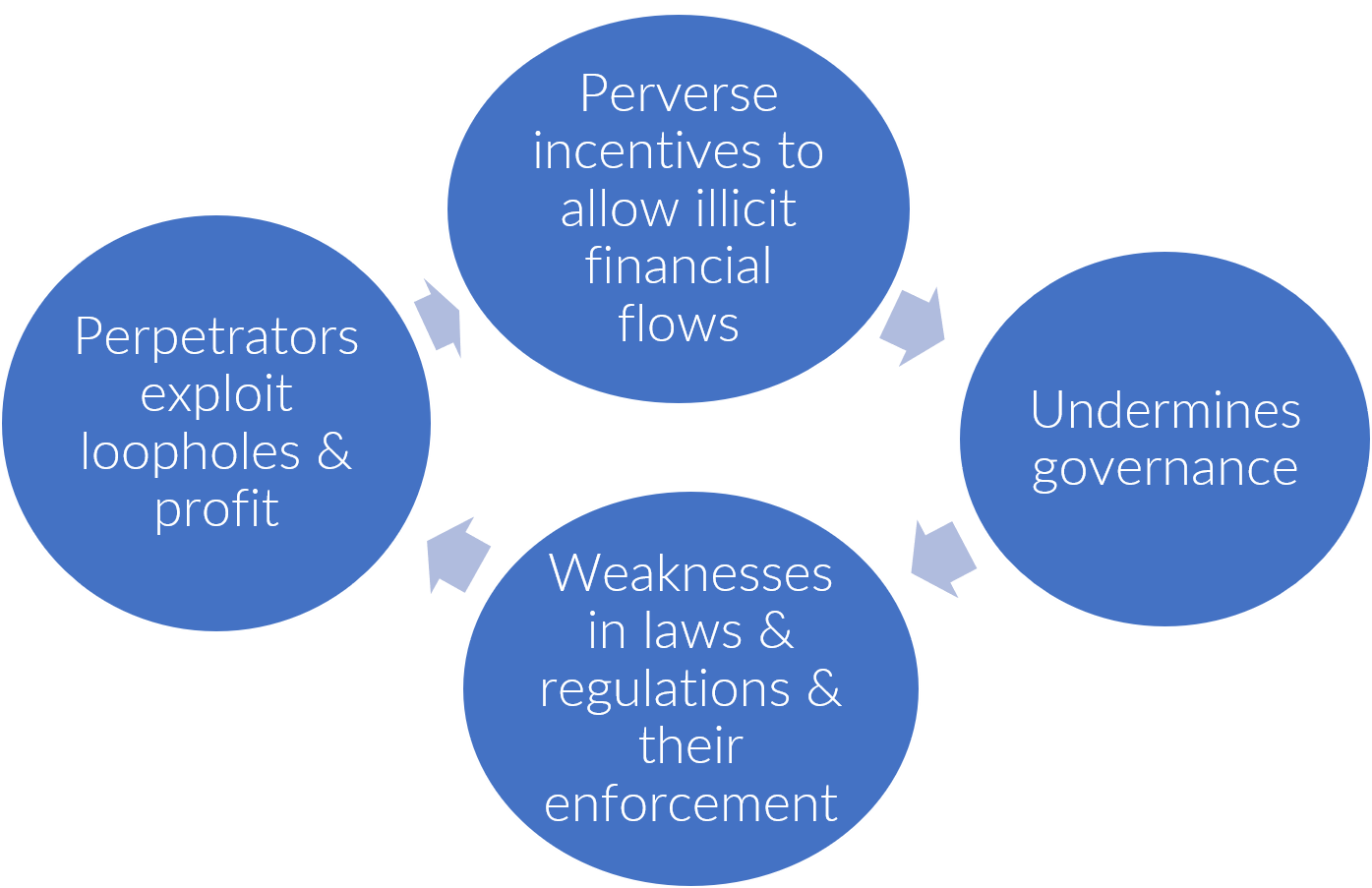 |
| Governance loop (credit: William Davis) |
Data source
Trade mis-invoicing data-set of the United Nations Economic Commission for Africa
Panel with \(n=6,248,254\) of mis-invoiced trade between 179 reporting jurisdictions and 179 partner countries for years 2000-2016 and disaggregated commodities
Citation: Lépissier, Alice, Davis, William, & Ibrahim, Gamal. (2019). Trade Mis-Invoicing Dataset (Version 1).

The entire data-set
panel_results.Rdatawith ~6 million observations is available online.The unit of observation is a reporter-partner-commodity-year tuple, where the data represent the illicit flow embedded in a transaction between a reporter \(i\) and a partner \(j\) for a commodity \(c\) in year \(t\).
The full panel is ~2GB. This notebook works with smaller summary data-sets generated from the full panel. The code to generate these summary data-sets is available on the repository https://github.com/walice/Trade-IFF by running the script file
Compute IFF Estimates.R.
Nota bene: the figures in this notebook that are not generated here can be reconstructed by running the Data Visualization.R script in that same repository.
Methodology for calculating mis-invoiced trade
We locate mis-invoicing in the discrepancies between reported trade flows and their mirrored statistics
But not all observed discrepancies are due to illicit motives!
Imports tend to be recorded on the basis of Cost of Insurance and Freight (CIF), while exports are recorded Free On Board (FOB)
Our approach
Estimate the discrepancies between imports and mirror net exports as a function of both licit and illicit predictors
Perform a harmonization procedure in order to generate a reconciled value that represents our best estimate of what the legitimate value of the trade should be on a FOB basis
Calculate the IFF embedded in each transaction as the difference between the observed value and the reconciled value
What this data-set represents
The data-set presents estimates of mis-invoicing both in imports and exports. I will be working with the import data.
There is a low and a high variant of mis-invoicing estimates. Discussion of how they vary is beyond the scope of this project, but note that we will be working with the high variant exclusively, as those are the official numbers of UNECA.
A negative value represents an illicit inflow, while a positive value represents an illicit outflow.
The panel can be aggregated over several dimensions, e.g. partner country, commodity, year. There are two methods to aggregate up the illicit flow:
Net basis: simply add up all negative and positive values, so that inflows and outflows cancel each other out
Gross Excluding Reversals (GER) basis: ignore all inflows, and sum up the positive values only across trading partners
Aggregation strategy
It is important to note that for a given country pair \(i\) and \(j\) in a given year \(t\), the same trade flow can be associated with either an inflow or an outflow according to what commodity is traded. While it might seem unlikely that illicit funds might be traveling in both directions for the same trade flow, there could be a variety of different actors doing this for different reasons. For example, country \(i\) might have export taxes on raw materials and export subsidies for manufacturing output, which would give an incentive to under-invoice exports of raw materials (resulting in an illicit outflow) and to over-invoice exports of manufactured goods (resulting in an illicit inflow). Alternatively, a criminal syndicate that has a legitimate front company may use re-invoicing to send money to an affiliate in another country to make an investment (e.g. hiring “muscle” to fight off a competitor) and then bring funds back using exports to the same country when the investment bears fruit.
The object of analytical inquiry should guide the choice of aggregation strategy. For example, stakeholders interested in getting a picture of the total amount of funds departing a country on balance should favor a net aggregation basis. By contrast, stakeholders interested in better understanding the drivers and mechanisms of IFF should favor aggregation using GER in order to identify where money is flowing out or in.
In this project, I will be using unsupervised machine learning to extract insights on analytically relevant dimensions of variation, so I will use summary data-sets that have been aggregated on a Gross Excluding Reversals basis. In other words, I am more interested in the direction and topology of the illicit flows, rather than their magnitude.
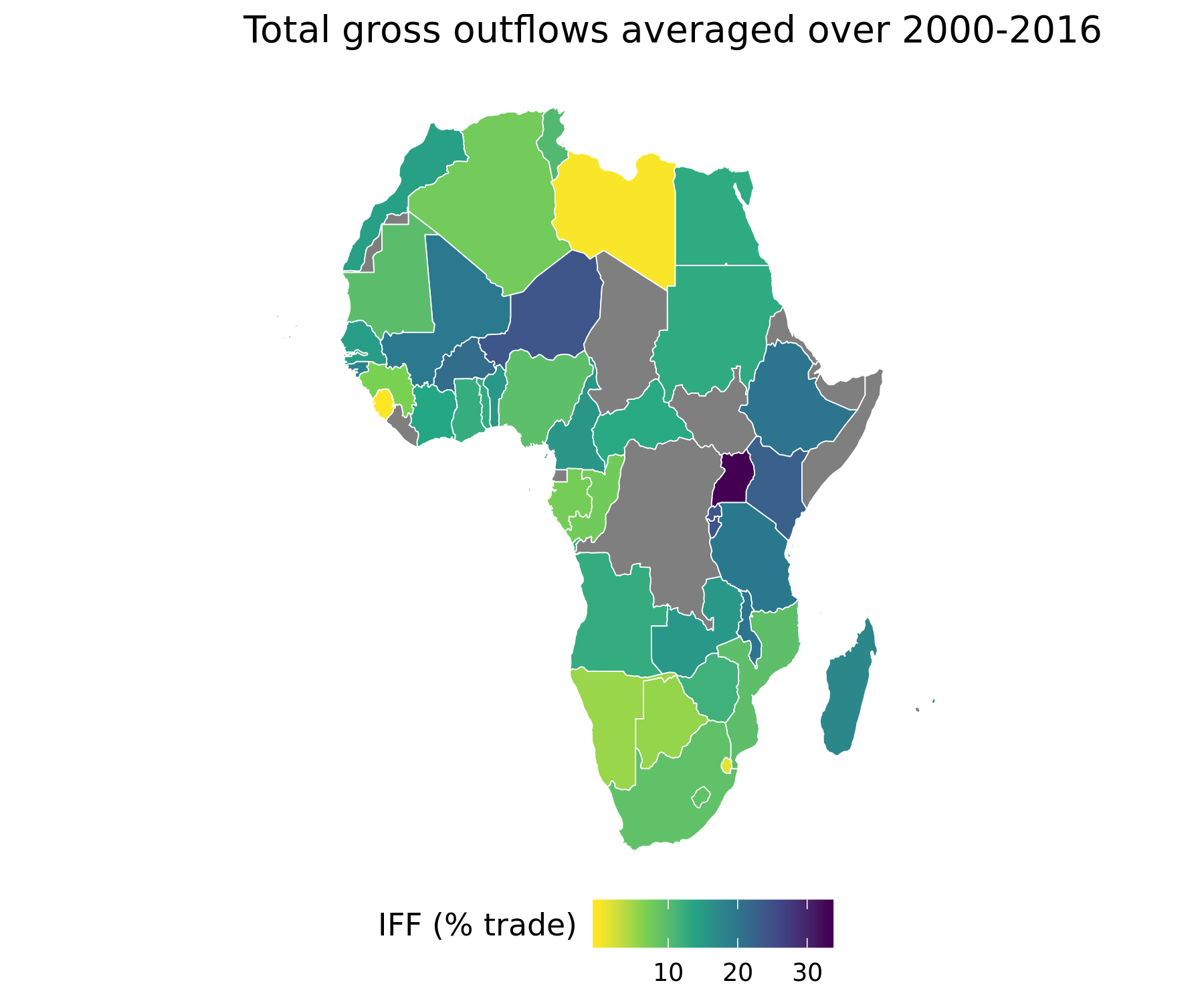
Zoom in on Africa
During 2000-2016, the continent lost on average $83 billion a year in gross illicit outflows
Net cumulative flows during that period were $362 billion
 Source: generated by
 Data Visualization.R in https://github.com/walice/Trade-IFF
Goals
While generating estimates of the dollar value of illicit trade has been helpful to shed light on the severity of the problem, the next step in the analysis is to further understand the nature of the illicit activity in terms of its origins, destinations, and sectors.
Therefore, the goal of this project is to extract meaningful insights on illicit trade using unsupervised machine learning techniques. By doing so, I can identify analytically relevant categories and dimensions of variation, in order to generate hypotheses and guide further work.
This project will apply the following techniques to the data:
Dimension reduction using Principal Components Analysis (PCA)
Clustering
Graph analysis
Data wrangling
I will work with two summary forms of the full data-set panel_results.Rdata: one where the data is aggregated up to the reporter country, and one where the dyadic nature of the data is preserved.
In the case where the data is aggregated up to the reporter country, there are two possible views of the feature space. On the one hand, the feature space can be spanned by the sectors of the different commodities (\(p=21\)). On the other hand, the feature space can be spanned by the reporter African countries (\(p=46\)).
Mis-invoiced trade for countries (aggregated data)
View 1: unit of observation = reporter-year; features = sectors
View 2: unit of observation = sector-year; features = reporters
Bilateral matrix of mis-invoiced trade (dyadic data)
Unit of observation = reporter-partner-year
Mis-invoiced trade data (for African reporting countries)
Let’s read in a summary data-set of the full panel which contains mis-invoicing estimates for reporter \(i\) in commodity \(c\) in year \(t\) (aggregated over partner countries \(j\) using the GER strategy).
IFF_Sector = pd.read_csv('Data/GER_Orig_Sect_Year_Africa.csv')
Let’s also extract the relevant labels for the countries in the data-set.
obs_info = IFF_Sector.reset_index().drop_duplicates(['reporter.ISO', 'year'])[['reporter.ISO',
'year',
'reporter',
'rIncome',
'rDev']]
obs_info = obs_info.replace({'LIC': 'Low income',
'LMC': 'Lower-middle income',
'UMC': 'Upper-middle income',
'HIC': 'High income'})
obs_info = obs_info.rename(columns={'rIncome': 'Income group (World Bank)',
'rDev': 'Country status (UN)'})
Mis-invoiced trade for countries by sectors
The table below displays the raw data of mis-invoiced trade for 46 African countries in 21 different sectors during 2000-2016, aggregated over partner countries.
| section | Imp_IFF_hi | ||
|---|---|---|---|
| reporter.ISO | year | ||
| DZA | 2001 | Animal and Animal Products | 1.914633e+08 |
| 2001 | Pulp of Wood or of Other Fibrous Material | 7.436143e+07 | |
| 2001 | Textiles | 3.560644e+07 | |
| 2001 | Footwear and Headgear | 1.146507e+06 | |
| 2001 | Stone, Glass, and Ceramics | 2.935880e+07 | |
| ... | ... | ... | ... |
| ZWE | 2007 | Arms and Ammunition | 0.000000e+00 |
| 2009 | Works of Art | 0.000000e+00 | |
| 2013 | Miscellaneous Manufactured Articles | 0.000000e+00 | |
| 2014 | Miscellaneous Manufactured Articles | 0.000000e+00 | |
| 2014 | Mineral Products | 0.000000e+00 |
11133 rows × 2 columns
Mis-invoiced trade data (bilateral trade matrix)
Now, let’s read in another summary data-set of the full panel which contains mis-invoicing estimates for reporter \(i\) with partner \(j\) in year \(t\) (aggregated over commodities \(c\) using the GER strategy).
IFF_Dest = pd.read_csv('Data/GER_Orig_Dest_Year_Africa.csv')
Mis-invoiced trade for dyads
The table below displays the raw data of mis-invoiced trade for 46 African countries with 167 partner countries during 2000-2016, aggregated over commodity sectors.
| partner.ISO | Imp_IFF_hi | ||
|---|---|---|---|
| reporter.ISO | year | ||
| DZA | 2001 | AND | 1.609561e+04 |
| 2001 | ARG | 4.717459e+07 | |
| 2001 | AUS | 2.027641e+07 | |
| 2001 | AUT | 7.641706e+07 | |
| 2001 | BEL | 2.285729e+07 | |
| ... | ... | ... | ... |
| ZWE | 2014 | MDG | 0.000000e+00 |
| 2014 | SGP | 0.000000e+00 | |
| 2014 | CHE | 0.000000e+00 | |
| 2014 | ARE | 0.000000e+00 | |
| 2015 | UGA | 0.000000e+00 |
34757 rows × 2 columns
Crosswalk data
Finally, let’s import a table that contains labels for the countries, such as their ISO codes, geographic regions, and income groupings that they belong to.
Metadata for countries
crosswalk = pd.read_excel("Data/crosswalk.xlsx").rename(columns={'Country': 'country'})
crosswalk.head()
| ISO3166.3 | ISO3166.2 | country | UN_Region | UN_Region_Code | UN_Sub-region | UN_Sub-region_Code | UN_Intermediate_Region | UN_Intermediate_Region_Code | UN_M49_Code | ... | WB_Income_Group_Code | WB_Region | WB_Lending_Category | WB_Other | OECD | EU28 | Arab League | Commonwealth | Longitude | Latitude | |
|---|---|---|---|---|---|---|---|---|---|---|---|---|---|---|---|---|---|---|---|---|---|
| 0 | ABW | AW | Aruba | Americas | 19.0 | Latin America and the Caribbean | 419.0 | Caribbean | 29.0 | 533.0 | ... | HIC | Latin America and Caribbean | .. | NaN | 0 | 0 | 0 | 0 | -69.982677 | 12.520880 |
| 1 | AFG | AF | Afghanistan | Asia | 142.0 | Southern Asia | 34.0 | NaN | NaN | 4.0 | ... | LIC | South Asia | IDA | HIPC | 0 | 0 | 0 | 0 | 66.004734 | 33.835231 |
| 2 | AFG | AF | Afghanistan, Islamic Republic of | Asia | 142.0 | Southern Asia | 34.0 | NaN | NaN | 4.0 | ... | LIC | South Asia | IDA | HIPC | 0 | 0 | 0 | 0 | 66.004734 | 33.835231 |
| 3 | AGO | AO | Angola | Africa | 2.0 | Sub-Saharan Africa | 202.0 | Middle Africa | 17.0 | 24.0 | ... | LMC | Sub-Saharan Africa | IBRD | NaN | 0 | 0 | 0 | 0 | 17.537368 | -12.293361 |
| 4 | AIA | AI | Anguila | Americas | 19.0 | Latin America and the Caribbean | 419.0 | Caribbean | 29.0 | 660.0 | ... | NaN | NaN | NaN | NaN | 0 | 0 | 0 | 0 | -63.064989 | 18.223959 |
5 rows × 25 columns
Auxiliary functions
I create three auxiliary functions to aid me in running Principal Component Analysis:
A function which creates the feature space for PCA from a data-set in a long format (which is the format of
IFF_SectorandIFF_Dest)A function which runs PCA and plots a biplot for two chosen principal components
A function which plots a cumulative scree plot
def create_features(data, values, features, obs):
"""
Convert data-set in long format to wide and preserve information on year.
data: {IFF_Sector_Imp, IFF_Dest_Imp, IFF_Dest_AFR, ...}, as Pandas dataframe,
name of data-set from which to create feature space, must be in long format
values: {'Imp_IFF_hi', 'Exp_IFF_hi'}, as string, values that data-set will represent
features: {'reporter.ISO', 'section', 'partner.ISO'}, as string,
what to use as the feature space
obs: {'section', 'reporter.ISO'}, as string, what to use as the observation level
"""
features_data = data.pivot_table(values=values,
columns=features,
index=[obs, 'year'],
fill_value=0)
return features_data
# Extra function to run the analysis on average mis-invoicing over the years
def create_features_mean(data, values, features, obs):
"""
Convert data-set in long format to wide.
data: {IFF_Sector_mean, IFF_Dest_mean, ...}, as Pandas dataframe,
name of data-set from which to create feature space, must be in long format
values: {'Imp_IFF_hi', 'Exp_IFF_hi'}, as string, values that data-set will represent
features: {'reporter.ISO', 'section', 'partner.ISO'}, as string,
what to use as the feature space
obs: {'section', 'reporter.ISO'}, as string, what to use as the observation level
"""
features_data = data.pivot_table(values=values,
columns=features,
index=obs,
fill_value=0)
return features_data
def biplot_PCA(features_data, nPC=2, firstPC=1, secondPC=2, obs='reporter.ISO', show_loadings=False):
"""
Project the data in the 2-dimensional space spanned by 2 principal components
chosen by the user, along with a bi-plot of the top 3 loadings per PC, and color observations
by class label.
Args:
features_data: as Pandas dataframe, data-set of features
nPC: number of principal components
firstPC: integer denoting first principal component to plot in bi-plot
secondPC: integer denoting second principal component to plot in bi-plot
obs: string denoting index of class labels (in features_data)
show_loadings: Boolean indicating whether PCA loadings should be displayed
Returns:
plot (interactive)
pca_loadings (if show_loadings=True)
"""
# Run PCA (standardize data beforehand)
features_data_std = StandardScaler().fit_transform(features_data)
pca = PCA(n_components=nPC, random_state=234)
princ_comp = pca.fit_transform(features_data_std)
# Extract PCA loadings
cols = ['PC' + str(c+1) for c in np.arange(nPC)]
pca_loadings = pd.DataFrame(pca.components_.T,
columns=cols,
index=list(features_data.columns))
# Extract PCA scores
pca_scores = pd.DataFrame(princ_comp,
columns=cols)
pca_scores[obs] = features_data.reset_index()[obs].values.tolist()
pca_scores['year'] = features_data.reset_index()['year'].values.tolist()
score_PC1 = princ_comp[:,firstPC-1]
score_PC2 = princ_comp[:,secondPC-1]
# Generate plot data
if obs == 'reporter.ISO':
plot_data = pd.merge(pca_scores, obs_info, on=[obs, 'year'])
color_obs = 'reporter'
tooltip_obs = ['reporter', 'year', 'Income group (World Bank)', 'Country status (UN)']
else:
plot_data = pca_scores
color_obs = 'section'
tooltip_obs = ['section', 'year']
# Return chosen PCs to plot
PC1 = 'PC'+str(firstPC)
PC2 = 'PC'+str(secondPC)
# Extract top loadings (in absolute value)
# TO DO: use dict to iterate over
toploadings_PC1 = pca_loadings.apply(lambda x: abs(x)).sort_values(by=PC1).tail(3)[[PC1, PC2]]
toploadings_PC2 = pca_loadings.apply(lambda x: abs(x)).sort_values(by=PC2).tail(3)[[PC1, PC2]]
originsPC1 = pd.DataFrame({'index':toploadings_PC1.index.tolist(),
PC1: np.zeros(3),
PC2: np.zeros(3)})
originsPC2 = pd.DataFrame({'index':toploadings_PC2.index.tolist(),
PC1: np.zeros(3),
PC2: np.zeros(3)})
toploadings_PC1 = pd.concat([toploadings_PC1.reset_index(), originsPC1], axis=0)
toploadings_PC2 = pd.concat([toploadings_PC2.reset_index(), originsPC2], axis=0)
toploadings_PC1[PC1] = toploadings_PC1[PC1]*max(score_PC1)*1.5
toploadings_PC1[PC2] = toploadings_PC1[PC2]*max(score_PC2)*1.5
toploadings_PC2[PC1] = toploadings_PC2[PC1]*max(score_PC1)*1.5
toploadings_PC2[PC2] = toploadings_PC2[PC2]*max(score_PC2)*1.5
# Project top 3 loadings over the space spanned by 2 principal components
lines = alt.Chart().mark_line().encode()
for color, i, dataset in zip(['#440154FF', '#21908CFF'], [0,1], [toploadings_PC1, toploadings_PC2]):
lines[i] = alt.Chart(dataset).mark_line(color=color).encode(
x= PC1 +':Q',
y= PC2 +':Q',
detail='index'
).properties(
width=400,
height=400
)
# Add labels to the loadings
text=alt.Chart().mark_text().encode()
for color, i, dataset in zip(['#440154FF', '#21908CFF'], [0, 1], [toploadings_PC1[0:3], toploadings_PC2[0:3]]):
text[i] = alt.Chart(dataset).mark_text(
align='left',
baseline='bottom',
color=color
).encode(
x= PC1 +':Q',
y= PC2 +':Q',
text='index'
)
# Scatter plot colored by observation class label
points = alt.Chart(plot_data).mark_circle(size=60).encode(
x=alt.X(PC1, axis=alt.Axis(title='Principal Component ' + str(firstPC))),
y=alt.X(PC2, axis=alt.Axis(title='Principal Component ' + str(secondPC))),
color=alt.Color(color_obs, scale=alt.Scale(scheme='category20b'),
legend=alt.Legend(orient='right')),
tooltip=tooltip_obs
).interactive()
# Bind it all together
chart = (points + lines[0] + lines[1] + text[0] + text[1])
chart.display()
if show_loadings:
return pca_loadings
def scree_plot(features_data, show_explained_var=False):
"""
Create a cumulative scree splot and (optional) return the explained variance by each component.
features_data: as Pandas dataframe, the data-set on which to run PCA
show_explained_var: as Boolean, flag for whether to return explained variance
"""
features_data_std = StandardScaler().fit_transform(features_data)
pca = PCA(n_components=features_data_std.shape[1], random_state=234)
princ_comp = pca.fit_transform(features_data_std)
explained_var = pd.DataFrame({'PC': np.arange(1,features_data_std.shape[1]+1),
'var': pca.explained_variance_ratio_,
'cumvar': np.cumsum(pca.explained_variance_ratio_)})
# Adapted from https://altair-viz.github.io/gallery/multiline_tooltip.html
# Create a selection that chooses the nearest point & selects based on x-value
nearest = alt.selection(type='single', nearest=True, on='mouseover',
fields=['PC'], empty='none')
# The basic line
line = alt.Chart(explained_var).mark_line(interpolate='basis', color='#FDE725FF').encode(
alt.X('PC:Q',
scale=alt.Scale(domain=(1, len(explained_var))),
axis=alt.Axis(title='Principal Component')
),
alt.Y('cumvar:Q',
scale=alt.Scale(domain=(min(explained_var['cumvar']), 1)),
axis=alt.Axis(title='Cumulative Variance Explained')
),
)
# Transparent selectors across the chart. This is what tells us
# the x-value of the cursor
selectors = alt.Chart(explained_var).mark_point().encode(
x='PC:Q',
opacity=alt.value(0),
).add_selection(
nearest
)
# Draw points on the line, and highlight based on selection
points = line.mark_point().encode(
opacity=alt.condition(nearest, alt.value(1), alt.value(0))
)
# Draw text labels near the points, and highlight based on selection
text = line.mark_text(align='left', dx=5, dy=-5).encode(
text=alt.condition(nearest, 'cumvar:Q', alt.value(' '))
)
# Draw a rule at the location of the selection
rules = alt.Chart(explained_var).mark_rule(color='gray').encode(
x='PC:Q',
).transform_filter(
nearest
)
# Put the five layers into a chart and bind the data
out = alt.layer(
line, selectors, points, rules, text
).properties(
title='Cumulative scree plot',
width=500, height=300
)
out.display()
if show_explained_var:
return explained_var[['PC', 'var']]
PCA on feature space (for individual reporting countries)
I now run PCA on the data-set IFF_Sector which includes mis-invoiced trade for a country \(i\) in commodity \(c\) in year \(t\).
Sector features
One possible view of IFF_Sector is to view the sectors as the feature space where \(p=21\). Therefore, I use the function create_features() to generate the data-set to be used in PCA analysis.
sector_features = create_features(IFF_Sector_Imp, 'Imp_IFF_hi',
features='section', obs='reporter.ISO')
sector_features
| section | Animal and Animal Products | Animal or Vegetable Fats and Oils | Arms and Ammunition | Base Metals | Chemicals and Allied Industries | Footwear and Headgear | Machinery and Electrical | Mineral Products | Miscellaneous Manufactured Articles | Pearls, Precious Stones and Metals | ... | Precision Instruments | Prepared Foodstuffs | Pulp of Wood or of Other Fibrous Material | Raw Hides, Skins, Leather, and Furs | Stone, Glass, and Ceramics | Textiles | Transportation | Vegetable Products | Wood and Wood Products | Works of Art | |
|---|---|---|---|---|---|---|---|---|---|---|---|---|---|---|---|---|---|---|---|---|---|---|
| reporter.ISO | year | |||||||||||||||||||||
| AGO | 2009 | 2.694946e+08 | 7.652455e+07 | 67738.261242 | 1.025920e+09 | 5.115176e+08 | 2.920410e+07 | 1.525512e+09 | 1.727293e+09 | 2.472936e+08 | 5.575633e+05 | ... | 1.242156e+08 | 4.781184e+08 | 1.149992e+08 | 1.097769e+07 | 1.349018e+08 | 1.827787e+08 | 2.198838e+09 | 4.249722e+08 | 4.337043e+07 | 177640.929155 |
| 2010 | 2.064906e+08 | 7.311396e+07 | 0.000000 | 9.989842e+08 | 2.575443e+08 | 7.853065e+06 | 1.308337e+09 | 2.953387e+09 | 8.404302e+07 | 3.209177e+05 | ... | 1.115183e+08 | 2.342889e+08 | 7.332134e+07 | 4.013044e+06 | 7.601278e+07 | 8.285704e+07 | 9.611656e+08 | 1.959128e+08 | 2.310136e+07 | 404828.231824 | |
| 2011 | 2.995594e+08 | 8.058180e+07 | 89365.880480 | 6.689511e+08 | 2.931591e+08 | 1.172881e+07 | 1.389743e+09 | 2.286539e+09 | 4.413341e+07 | 9.645181e+05 | ... | 1.418956e+08 | 3.159980e+08 | 9.911835e+07 | 9.995669e+06 | 6.607126e+07 | 7.912925e+07 | 7.070474e+08 | 3.734589e+08 | 1.363601e+07 | 586586.948365 | |
| 2012 | 7.103770e+08 | 2.746924e+08 | 261265.895948 | 1.753970e+09 | 8.540407e+08 | 3.823724e+07 | 2.790368e+09 | 9.203666e+08 | 1.763904e+08 | 1.271289e+06 | ... | 2.073111e+08 | 1.025668e+09 | 2.641831e+08 | 1.394356e+07 | 1.630307e+08 | 1.683128e+08 | 1.975553e+09 | 6.541154e+08 | 3.980884e+07 | 739122.050820 | |
| 2013 | 4.031560e+08 | 1.541679e+08 | 188343.533148 | 9.230300e+08 | 4.793908e+08 | 1.212363e+07 | 1.428283e+09 | 2.009915e+09 | 4.871315e+07 | 6.250082e+05 | ... | 1.063123e+08 | 4.931687e+08 | 1.798533e+08 | 8.930246e+06 | 7.882264e+07 | 7.858108e+07 | 4.962937e+09 | 3.995114e+08 | 1.836680e+07 | 418841.640492 | |
| ... | ... | ... | ... | ... | ... | ... | ... | ... | ... | ... | ... | ... | ... | ... | ... | ... | ... | ... | ... | ... | ... | ... |
| ZWE | 2011 | 3.098093e+07 | 6.060789e+07 | 9124.882478 | 1.693777e+08 | 2.260227e+09 | 2.817909e+06 | 3.231869e+08 | 2.747704e+08 | 9.872441e+06 | 3.618592e+06 | ... | 2.136919e+07 | 1.144497e+08 | 5.855387e+07 | 6.259512e+05 | 2.652474e+07 | 4.726781e+07 | 8.963644e+08 | 1.874874e+08 | 6.016952e+06 | 35481.251510 |
| 2012 | 2.784481e+07 | 5.549232e+07 | 856.631347 | 1.085453e+08 | 4.929549e+08 | 7.015919e+06 | 3.451931e+08 | 1.461844e+08 | 1.510668e+07 | 2.876014e+05 | ... | 3.162707e+07 | 2.025934e+08 | 6.024629e+07 | 1.412797e+06 | 2.482629e+07 | 5.147542e+07 | 9.468142e+08 | 1.900125e+08 | 7.901902e+06 | 59677.045599 | |
| 2013 | 0.000000e+00 | 0.000000e+00 | 0.000000 | 0.000000e+00 | 0.000000e+00 | 0.000000e+00 | 0.000000e+00 | 0.000000e+00 | 0.000000e+00 | 0.000000e+00 | ... | 0.000000e+00 | 0.000000e+00 | 0.000000e+00 | 0.000000e+00 | 0.000000e+00 | 0.000000e+00 | 0.000000e+00 | 0.000000e+00 | 0.000000e+00 | 0.000000 | |
| 2014 | 0.000000e+00 | 0.000000e+00 | 0.000000 | 0.000000e+00 | 0.000000e+00 | 0.000000e+00 | 0.000000e+00 | 0.000000e+00 | 0.000000e+00 | 0.000000e+00 | ... | 0.000000e+00 | 0.000000e+00 | 0.000000e+00 | 0.000000e+00 | 0.000000e+00 | 0.000000e+00 | 0.000000e+00 | 0.000000e+00 | 0.000000e+00 | 0.000000 | |
| 2015 | 1.458046e+07 | 7.135043e+07 | 19192.507302 | 8.703951e+07 | 2.299085e+08 | 4.468801e+06 | 3.437244e+08 | 1.401916e+08 | 2.432263e+07 | 3.672531e+07 | ... | 3.233606e+07 | 3.778318e+07 | 3.157795e+07 | 1.061420e+06 | 1.724449e+07 | 2.841926e+07 | 2.137692e+08 | 1.585549e+08 | 4.569325e+06 | 6305.070602 |
624 rows × 21 columns
Biplots
The figure below displays a biplot of the first 2 principal components, in addition to reporting the loadings for all principal components in the following table.
biplot_PCA(sector_features, 10, 1, 2, obs='reporter.ISO', show_loadings=True)
| PC1 | PC2 | PC3 | PC4 | PC5 | PC6 | PC7 | PC8 | PC9 | PC10 | |
|---|---|---|---|---|---|---|---|---|---|---|
| Animal and Animal Products | 0.223097 | -0.285686 | -0.052218 | 0.200337 | 0.280789 | -0.075192 | -0.159824 | 0.157986 | -0.133621 | 0.067581 |
| Animal or Vegetable Fats and Oils | 0.145805 | -0.041750 | 0.262100 | -0.281551 | -0.378544 | -0.470151 | 0.409970 | 0.471670 | 0.177591 | -0.031639 |
| Arms and Ammunition | 0.030559 | -0.044358 | 0.524677 | -0.654182 | 0.434354 | 0.055627 | -0.201368 | -0.113006 | -0.079142 | -0.115541 |
| Base Metals | 0.235966 | -0.206534 | -0.261180 | -0.147777 | -0.019680 | -0.153272 | 0.017922 | -0.247084 | 0.174715 | -0.069873 |
| Chemicals and Allied Industries | 0.271238 | 0.107591 | -0.117222 | -0.089472 | -0.096976 | -0.130645 | -0.071165 | -0.219172 | -0.198166 | 0.036517 |
| Footwear and Headgear | 0.206357 | 0.378112 | 0.015170 | -0.019961 | -0.001383 | -0.029500 | -0.042735 | 0.010544 | 0.026510 | -0.252435 |
| Machinery and Electrical | 0.272101 | 0.160466 | 0.076229 | 0.091921 | -0.067637 | -0.159494 | 0.022549 | -0.135941 | -0.157103 | -0.115312 |
| Mineral Products | 0.238785 | 0.071925 | -0.098357 | -0.201011 | -0.166463 | 0.073908 | -0.133348 | 0.121464 | -0.241190 | 0.675042 |
| Miscellaneous Manufactured Articles | 0.246123 | 0.283544 | 0.122775 | 0.033592 | -0.049743 | -0.014818 | -0.017630 | 0.069480 | -0.247438 | -0.043076 |
| Pearls, Precious Stones and Metals | 0.060193 | 0.251657 | -0.373387 | -0.153599 | 0.567863 | 0.055855 | 0.647708 | 0.088517 | -0.049224 | 0.089860 |
| Plastics and Rubbers | 0.264093 | -0.144764 | 0.124109 | 0.236111 | 0.112342 | 0.023331 | 0.062706 | 0.076398 | 0.119468 | -0.076649 |
| Precision Instruments | 0.223754 | 0.362288 | -0.013533 | 0.023957 | -0.084425 | -0.090796 | -0.080419 | -0.186415 | -0.262231 | -0.078130 |
| Prepared Foodstuffs | 0.252722 | -0.227483 | -0.012139 | 0.160146 | 0.177798 | -0.024717 | -0.088546 | 0.289203 | -0.187744 | -0.058613 |
| Pulp of Wood or of Other Fibrous Material | 0.272304 | -0.112890 | -0.010570 | 0.074023 | 0.024044 | -0.016865 | 0.003323 | -0.123810 | 0.135842 | 0.200798 |
| Raw Hides, Skins, Leather, and Furs | 0.206454 | 0.084348 | 0.178427 | 0.121865 | -0.101317 | 0.619649 | 0.102592 | 0.287981 | -0.057302 | -0.251296 |
| Stone, Glass, and Ceramics | 0.225603 | 0.111290 | 0.264504 | 0.269760 | 0.061210 | -0.018303 | 0.176815 | -0.368090 | 0.400752 | -0.018317 |
| Textiles | 0.209936 | -0.103101 | -0.054321 | -0.264334 | -0.273480 | 0.542184 | 0.126078 | -0.076346 | 0.216014 | 0.139611 |
| Transportation | 0.238443 | -0.119628 | 0.256225 | 0.081261 | 0.184539 | -0.059237 | 0.015553 | -0.095856 | 0.219874 | 0.334486 |
| Vegetable Products | 0.245486 | -0.284943 | -0.122225 | -0.029458 | 0.071482 | -0.036325 | -0.074223 | 0.202113 | -0.106308 | -0.240274 |
| Wood and Wood Products | 0.201178 | -0.222154 | -0.377723 | -0.300290 | -0.132165 | 0.007197 | -0.048891 | -0.185469 | 0.074259 | -0.351532 |
| Works of Art | 0.089055 | 0.388758 | -0.239308 | -0.078967 | 0.157495 | -0.041382 | -0.486227 | 0.369405 | 0.561157 | 0.018339 |
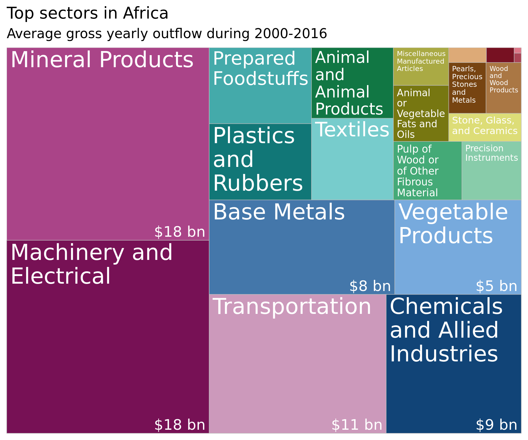
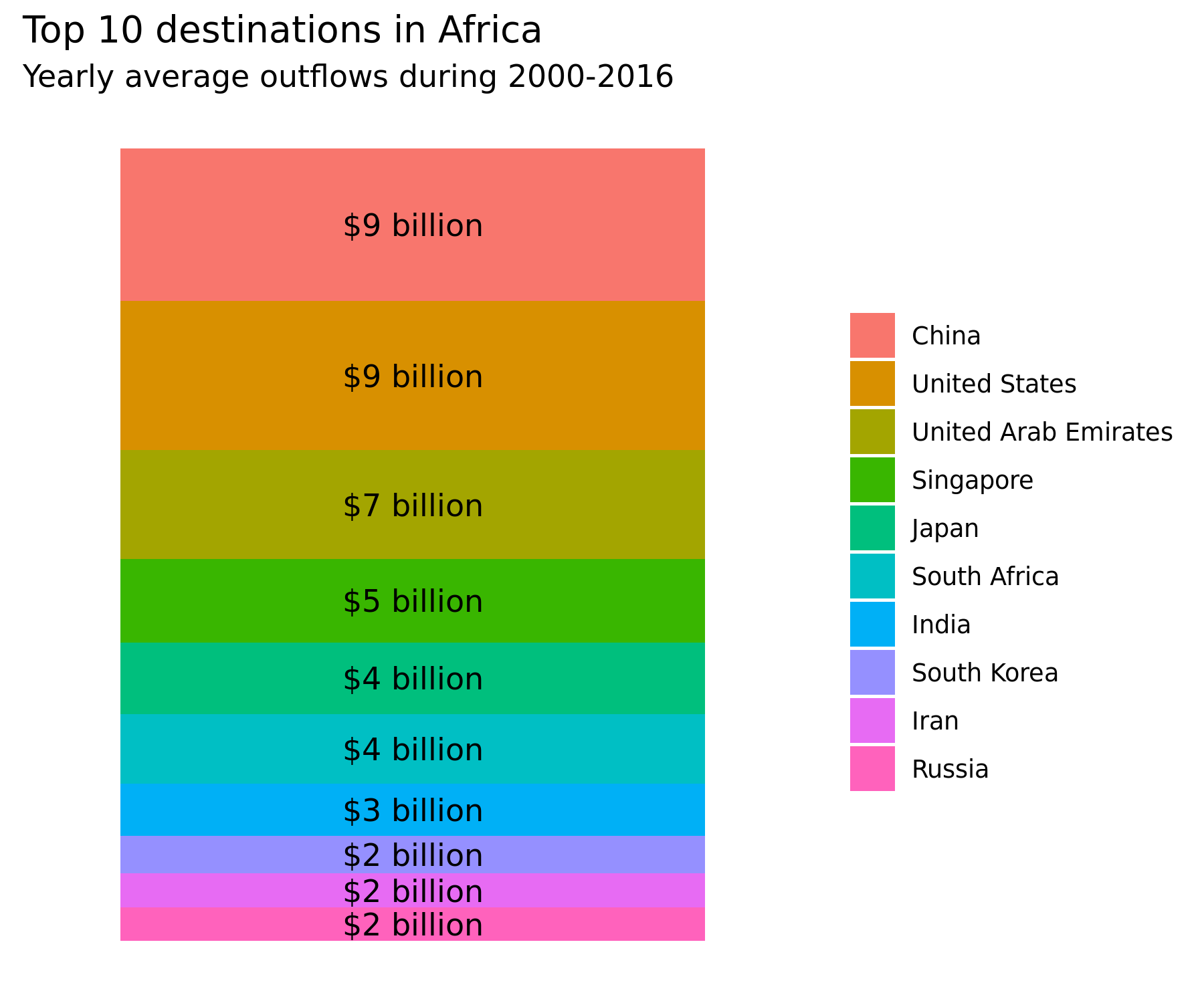
The first two principal components can be interpreted as recovering variation in the size of the illicit flow. The top loadings on the first principal component include Machinery and Electrical, and Chemicals and Allied Industries, which are the sectors with the highest amount of mis-invoiced trade. The treemap figure below represents the average gross yearly outflow to different sectors in Africa, and we can see that the aforementioned sectors account for a large chunk of that.
By contrast, the loadings on the second component are associated with sectors which are specialized, precision sectors that do not account for a large amount of mis-invoicing, compared to others. Indeed, Works of Art, and Footwear and Headgear are in the top-right corner of the treemap figure (and do not even appear with labels as they are so small).
Thus, it seems like the magnitude of the trade mis-invoicing (in dollar values) explains the highest variability in the data.
 Source: generated by
 Data Visualization.R in https://github.com/walice/Trade-IFF
biplot_PCA(sector_features, 10, 3, 4, obs='reporter.ISO')
The sixth principal component (displayed in the figure below) captures variation with respect to the natural origin of the commodity being traded and its functional use. The top loadings include sectors where the commodity is generated from natural resources (e.g. animals or vegetables) and which is functionally used in clothing, cooking, and cosmetics (e.g. textiles, leathers, oils).
biplot_PCA(sector_features, 10, 5, 6, obs='reporter.ISO')
Explained variance
The first 6 principal components examined above explain 83% of the variance in the data. The first principal component, which captures magnitude of the flow, accounts of 52% of the variance alone.
scree_plot(sector_features, show_explained_var=True)
| PC | var | |
|---|---|---|
| 0 | 1 | 0.524988 |
| 1 | 2 | 0.121415 |
| 2 | 3 | 0.054159 |
| 3 | 4 | 0.049898 |
| 4 | 5 | 0.042107 |
| 5 | 6 | 0.041007 |
| 6 | 7 | 0.036014 |
| 7 | 8 | 0.028847 |
| 8 | 9 | 0.024146 |
| 9 | 10 | 0.018279 |
| 10 | 11 | 0.012558 |
| 11 | 12 | 0.009987 |
| 12 | 13 | 0.007011 |
| 13 | 14 | 0.006890 |
| 14 | 15 | 0.005213 |
| 15 | 16 | 0.004848 |
| 16 | 17 | 0.004001 |
| 17 | 18 | 0.002819 |
| 18 | 19 | 0.002489 |
| 19 | 20 | 0.001800 |
| 20 | 21 | 0.001524 |
Variance-stabilizing and normalizing transformations
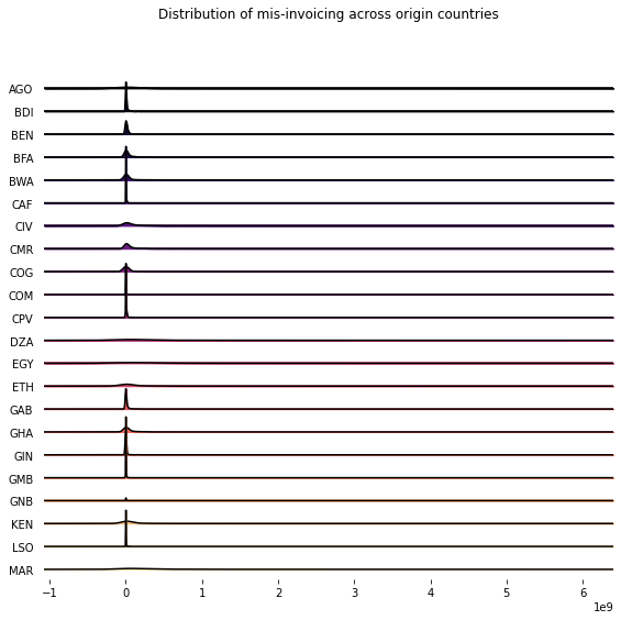
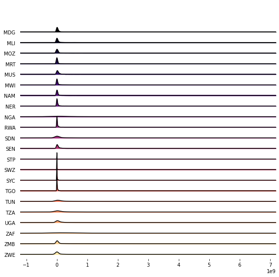
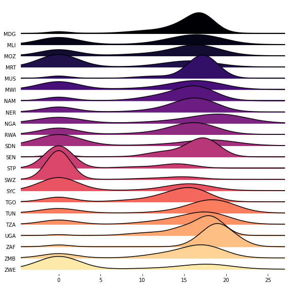
The figure below displays the distribution of mis-invoicing for the 21 different sectors. It is heavily right-skewed across all sectors, with very few high-value mis-invoiced transactions.
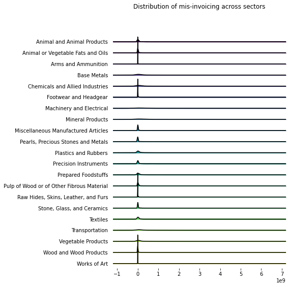
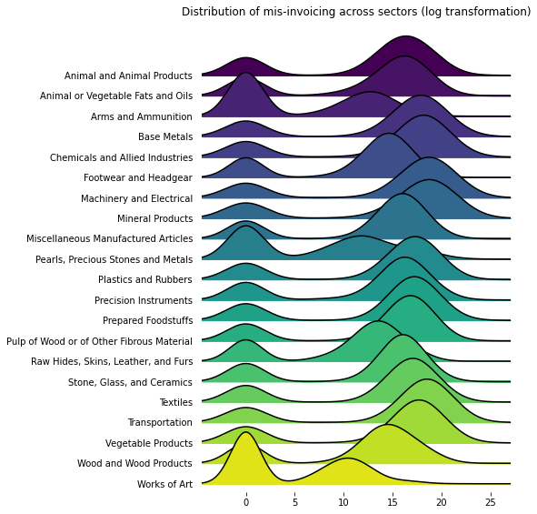
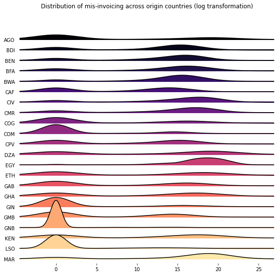
I explore two possible transformations of the data: a (modified) log transformation and a Yeo–Johnson. The values of the data-set are all non-negative, with some values equal to 0. Therefore, the figure below displays the distribution of the data after taking \(log(x+1)\).
sector_features_log = sector_features.apply(lambda x: np.log(x+1) if np.issubdtype(x.dtype, np.number) else x, axis=0)
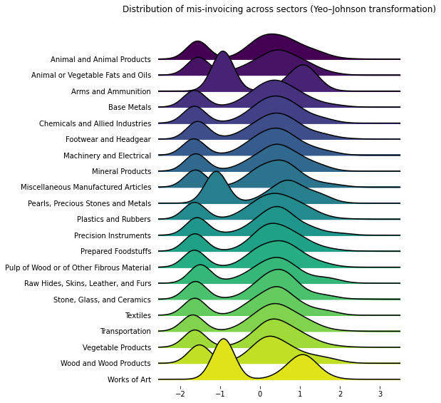
The Yeo-Johnson transformation is similar to a Box-Cox transformation, but allows for zero values. When \(x=0\) and the tuning parameter \(\lambda=0\), it will apply the same modified log transformation, \(log(x=1)\), as described above.
sector_features_yeo = power_transform(sector_features, method='yeo-johnson', standardize=True)
sector_features_yeo = pd.DataFrame(sector_features_yeo,
index=sector_features.index,
columns=sector_features.columns)
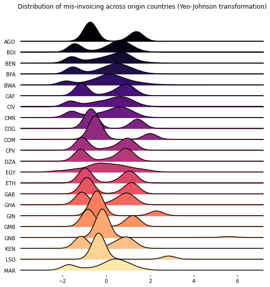
fig, axes = joypy.joyplot(sector_features_yeo, colormap=plt.cm.viridis, figsize=(8,8),
title='Distribution of mis-invoicing across sectors (Yeo–Johnson transformation)');
The two figures below display the results of running the PCA analysis on transformations of the data using a modified log and a Yeo-Johnson transformation, respectively.
The top loadings on the second principal component are the same and refer to Works of Art, Pearls, Precious Stones and Metals, and Arms and Ammunitions. These sectors refer to extremely high value-added sectors where the traded commodity is a finished product.
By contrast, the loadings on the first principal component (in either transformation) refer to heavy industries, where the commodity is an intermediate product (as opposed to a finished product). Even after applying normalizing transformations, the first principal component recovers sectors which were responsible for a large amount of the dollar value of mis-invoicing in the continent during 2000-2016.
biplot_PCA(sector_features_log, 10, 1, 2, obs='reporter.ISO')
biplot_PCA(sector_features_yeo, 10, 1, 2, obs='reporter.ISO')
Finally, transforming the data improves the performance of the PCA analysis, in the sense that the first two principal components now explain 90% of the variance in the data.
scree_plot(sector_features_yeo)
Country features
The second view of IFF_Sector is to consider the reporter countries as the feature space. Below, I use the function create_features() and specify reporter.ISO as the features in order to generate the data-set for PCA. In this case, we have \(p=46\).
The interpretation in this application is to understand the variation in where the illicit outflows originate. This is because the values have been aggregated using the GER strategy which captures outflows only.
country_features = create_features(IFF_Sector_Imp, 'Imp_IFF_hi',
features='reporter.ISO', obs='section')
country_features
| reporter.ISO | AGO | BDI | BEN | BFA | BWA | CAF | CIV | CMR | COG | COM | ... | STP | SWZ | SYC | TGO | TUN | TZA | UGA | ZAF | ZMB | ZWE | |
|---|---|---|---|---|---|---|---|---|---|---|---|---|---|---|---|---|---|---|---|---|---|---|
| section | year | |||||||||||||||||||||
| Animal and Animal Products | 2000 | 0.000000 | 0.000000 | 0.000000e+00 | 0.000000e+00 | 0.000000e+00 | 0.000000 | 0.000000e+00 | 0.000000e+00 | 0.00000 | 0.0 | ... | 0.000000 | 0.000000 | 0.000000e+00 | 4.044600e+06 | 1.572640e+07 | 1.060197e+06 | 2.902091e+05 | 2.341209e+07 | 0.000000e+00 | 0.000000e+00 |
| 2001 | 0.000000 | 0.000000 | 9.464068e+06 | 2.013378e+06 | 4.018742e+06 | 351958.882652 | 7.103384e+07 | 2.552567e+07 | 0.00000 | 0.0 | ... | 0.000000 | 0.000000 | 3.439935e+07 | 1.087398e+07 | 0.000000e+00 | 0.000000e+00 | 2.522664e+05 | 1.854458e+07 | 1.832385e+06 | 0.000000e+00 | |
| 2002 | 0.000000 | 288779.572593 | 1.458450e+07 | 7.756380e+05 | 3.524820e+06 | 213560.077651 | 7.767896e+07 | 2.907597e+07 | 0.00000 | 0.0 | ... | 0.000000 | 0.000000 | 0.000000e+00 | 6.574580e+06 | 9.664435e+06 | 0.000000e+00 | 6.944404e+05 | 1.452489e+07 | 4.354400e+05 | 7.346496e+06 | |
| 2003 | 0.000000 | 217920.960357 | 2.297721e+07 | 4.533317e+05 | 0.000000e+00 | 0.000000 | 1.286866e+08 | 3.485783e+07 | 0.00000 | 0.0 | ... | 0.000000 | 0.000000 | 0.000000e+00 | 6.290272e+06 | 1.732785e+07 | 1.294665e+06 | 1.358896e+06 | 2.153838e+07 | 1.422125e+06 | 0.000000e+00 | |
| 2004 | 0.000000 | 0.000000 | 2.742553e+07 | 3.429694e+05 | 5.275531e+04 | 0.000000 | 9.283012e+07 | 4.940023e+07 | 0.00000 | 0.0 | ... | 0.000000 | 59632.763605 | 0.000000e+00 | 3.901862e+06 | 3.574647e+07 | 0.000000e+00 | 8.053124e+05 | 2.868016e+07 | 2.791570e+06 | 0.000000e+00 | |
| ... | ... | ... | ... | ... | ... | ... | ... | ... | ... | ... | ... | ... | ... | ... | ... | ... | ... | ... | ... | ... | ... | ... |
| Works of Art | 2012 | 739122.050820 | 0.000000 | 0.000000e+00 | 1.054676e+04 | 2.623004e+05 | 0.000000 | 1.820478e+04 | 3.875133e+05 | 0.00000 | 0.0 | ... | 0.000000 | 0.000000 | 0.000000e+00 | 1.125696e+03 | 0.000000e+00 | 7.252236e+04 | 1.388514e+04 | 1.371564e+07 | 3.453691e+04 | 5.967705e+04 |
| 2013 | 418841.640492 | 0.000000 | 0.000000e+00 | 0.000000e+00 | 2.282032e+04 | 0.000000 | 1.287629e+04 | 2.104949e+04 | 0.00000 | 0.0 | ... | 9584.734907 | 0.000000 | 0.000000e+00 | 0.000000e+00 | 0.000000e+00 | 5.191721e+05 | 2.986963e+04 | 1.006657e+07 | 1.017682e+05 | 0.000000e+00 | |
| 2014 | 390140.730849 | 0.000000 | 0.000000e+00 | 0.000000e+00 | 9.331590e+04 | 0.000000 | 1.017252e+06 | 1.826816e+05 | 8003.37246 | 0.0 | ... | 20941.755221 | 0.000000 | 0.000000e+00 | 0.000000e+00 | 0.000000e+00 | 6.731774e+04 | 2.129568e+04 | 2.543377e+07 | 0.000000e+00 | 0.000000e+00 | |
| 2015 | 0.000000 | 0.000000 | 0.000000e+00 | 0.000000e+00 | 5.977903e+04 | 0.000000 | 0.000000e+00 | 0.000000e+00 | 0.00000 | 0.0 | ... | 4447.368931 | 0.000000 | 5.857979e+05 | 0.000000e+00 | 3.088086e+03 | 5.385830e+05 | 1.193596e+04 | 6.697451e+06 | 5.843484e+04 | 6.305071e+03 | |
| 2016 | 0.000000 | 0.000000 | 0.000000e+00 | 0.000000e+00 | 4.195233e+04 | 0.000000 | 0.000000e+00 | 0.000000e+00 | 0.00000 | 0.0 | ... | 1327.652396 | 0.000000 | 4.463501e+05 | 0.000000e+00 | 0.000000e+00 | 3.443084e+04 | 2.305443e+03 | 1.295357e+07 | 0.000000e+00 | 0.000000e+00 |
357 rows × 46 columns
Biplots
The three figures below display biplots for the first and second principal components, for the third and fourth principal components, and for the fifth and sixth principal components, respectively. The loadings for each reporter country are also reported.
biplot_PCA(country_features, 10, 1, 2, obs='section', show_loadings=True)
| PC1 | PC2 | PC3 | PC4 | PC5 | PC6 | PC7 | PC8 | PC9 | PC10 | |
|---|---|---|---|---|---|---|---|---|---|---|
| AGO | 0.172866 | 5.695754e-02 | 1.915290e-01 | -6.571267e-02 | -1.498597e-02 | 2.683983e-01 | -6.131957e-02 | -9.901379e-02 | -1.352142e-02 | 1.960619e-01 |
| BDI | 0.159396 | 1.399172e-02 | 1.100982e-01 | 1.072287e-01 | -5.780584e-02 | -3.006342e-02 | 1.311807e-01 | -6.306715e-02 | 8.380471e-02 | -1.595603e-01 |
| BEN | 0.166261 | 2.839527e-01 | -4.853377e-02 | -1.227506e-01 | -8.929173e-02 | 2.840864e-02 | -5.069704e-02 | -1.050768e-01 | 1.115173e-01 | -1.479526e-01 |
| BFA | 0.200912 | 1.961349e-01 | -1.479219e-02 | -3.284903e-02 | -7.687652e-03 | 1.947496e-01 | -8.961797e-03 | -9.812748e-02 | 5.298346e-02 | -6.100222e-02 |
| BWA | 0.058704 | 5.101605e-04 | 1.048248e-01 | 1.176491e-01 | 1.116177e-01 | 4.542630e-02 | 5.291913e-02 | 1.702242e-01 | 1.074927e-01 | 6.990029e-01 |
| CAF | 0.136213 | -2.941790e-01 | 7.144585e-02 | 1.466869e-01 | 1.005191e-01 | -8.211151e-04 | 1.767076e-02 | -9.841998e-02 | 4.459720e-02 | -6.455230e-02 |
| CIV | 0.170157 | -4.190252e-02 | -1.992766e-01 | -1.178971e-01 | -8.139640e-02 | 2.099028e-01 | 1.481461e-01 | -9.124417e-02 | 9.430036e-02 | -2.959315e-02 |
| CMR | 0.199563 | 6.685309e-03 | 2.723196e-02 | -1.591573e-01 | -1.158744e-01 | 4.651018e-02 | 4.997217e-02 | -4.900403e-02 | 6.736277e-02 | -4.601119e-02 |
| COG | 0.092230 | -1.314851e-01 | 3.146417e-01 | -1.361157e-01 | -2.737181e-01 | 2.682128e-01 | -4.522047e-02 | 1.802042e-02 | 4.328099e-02 | 3.111778e-02 |
| COM | 0.096409 | -2.063490e-01 | 2.921122e-01 | -2.226963e-01 | -7.053853e-02 | -1.456883e-01 | 8.379586e-02 | -6.576844e-02 | 9.280223e-02 | -1.472937e-01 |
| CPV | 0.162562 | -1.932140e-01 | 3.911200e-02 | -6.076881e-02 | 6.992487e-02 | 3.542767e-02 | 2.890140e-01 | -1.259045e-01 | 5.085305e-02 | -4.426356e-02 |
| DZA | 0.097941 | 4.125012e-02 | -3.694645e-02 | 4.185959e-01 | -2.291923e-01 | -2.224267e-01 | -7.905464e-02 | 8.880404e-02 | -9.011562e-02 | -5.841375e-02 |
| EGY | 0.175564 | 1.852732e-01 | 9.778806e-02 | 1.870187e-01 | 8.946189e-03 | -2.924499e-03 | 1.181851e-02 | -4.328654e-02 | 4.339753e-03 | -1.929171e-01 |
| ETH | 0.121994 | -1.897909e-01 | 7.695418e-02 | 3.167105e-01 | 2.484336e-01 | -1.802844e-01 | -7.872203e-02 | -9.597359e-02 | -2.026803e-02 | -1.094738e-01 |
| GAB | 0.042052 | -1.989049e-01 | -3.375917e-01 | 1.247060e-02 | -2.588424e-01 | -4.558121e-02 | 8.313195e-02 | 9.621236e-02 | -7.997286e-02 | -1.514322e-01 |
| GHA | 0.107784 | -1.996829e-01 | -6.503997e-02 | 6.007675e-02 | -3.272539e-01 | 2.451643e-01 | 4.926298e-02 | 2.807364e-01 | -3.340735e-01 | -5.059900e-03 |
| GIN | 0.052400 | -1.350973e-01 | -3.351174e-01 | -8.155761e-02 | -4.401417e-02 | -4.334381e-02 | -3.444465e-01 | -1.967460e-02 | 1.193137e-01 | -2.723141e-02 |
| GMB | 0.162689 | 8.598690e-02 | -9.929674e-02 | -2.316451e-01 | 2.262847e-01 | 1.330992e-01 | 2.662606e-01 | 1.742886e-01 | -9.401992e-02 | -6.012329e-02 |
| GNB | 0.000016 | -1.996604e-02 | -8.847847e-02 | -2.131943e-02 | 6.445089e-02 | 9.726163e-02 | -2.861441e-01 | 3.631337e-01 | 5.592464e-01 | -2.128313e-01 |
| KEN | 0.117135 | -1.733487e-01 | -2.826062e-01 | -1.414929e-01 | -4.852900e-02 | 1.122855e-01 | -1.773947e-01 | -2.061400e-01 | -2.190356e-01 | 1.721080e-01 |
| LBY | 0.000000 | 0.000000e+00 | -0.000000e+00 | 1.654361e-24 | 1.355253e-20 | 0.000000e+00 | 0.000000e+00 | 2.081668e-17 | -2.220446e-16 | -9.714451e-17 |
| LSO | 0.031001 | -1.145362e-01 | 1.172217e-01 | -8.783260e-02 | -6.316290e-02 | 1.845925e-01 | -1.155909e-01 | 4.273390e-01 | 1.846813e-01 | -2.597209e-02 |
| MAR | 0.196450 | -1.442017e-03 | -1.407898e-01 | -1.151253e-01 | 4.096951e-02 | -2.501230e-01 | -1.218791e-01 | -1.159986e-01 | -2.772756e-02 | 9.286997e-02 |
| MDG | 0.187159 | 1.768800e-01 | -7.603241e-02 | 1.954600e-02 | 3.882583e-02 | -6.632947e-02 | 1.303028e-02 | 1.697959e-01 | 3.997142e-02 | -1.389174e-01 |
| MLI | 0.160911 | -1.212446e-01 | -4.690084e-02 | -1.486856e-01 | 8.742975e-02 | -2.762972e-01 | 8.729569e-02 | 2.434701e-01 | -8.316575e-02 | 3.368757e-02 |
| MOZ | 0.147230 | 1.608981e-01 | 9.473738e-02 | -1.983947e-02 | -2.406356e-01 | -2.654582e-01 | -2.507807e-03 | 5.991142e-02 | 9.261240e-02 | 1.184466e-01 |
| MRT | 0.142351 | 2.001775e-01 | 7.014463e-02 | -1.332407e-01 | -2.101042e-01 | -3.003770e-01 | -1.237907e-01 | -9.258926e-02 | 7.149717e-02 | 1.249696e-01 |
| MUS | 0.183529 | 7.441746e-02 | -1.253785e-01 | 7.372575e-02 | 1.275615e-01 | 4.308231e-02 | 8.698864e-02 | 1.594759e-01 | 3.117765e-02 | 8.570793e-02 |
| MWI | 0.196370 | 1.208545e-01 | -1.804584e-02 | -1.462830e-01 | 2.430288e-02 | 7.000297e-02 | -7.395843e-02 | -3.780468e-02 | -6.553461e-02 | -1.841761e-02 |
| NAM | 0.173960 | 1.201903e-01 | 5.978034e-02 | 9.556719e-02 | 2.108371e-01 | -2.454492e-02 | 2.251590e-01 | 1.968563e-01 | -5.019903e-04 | 1.281223e-01 |
| NER | 0.191899 | -1.071062e-01 | 1.036822e-01 | -3.490165e-02 | 8.799988e-03 | 4.101665e-02 | -1.036213e-01 | -1.501394e-01 | 5.717845e-02 | 7.629436e-02 |
| NGA | 0.153000 | -8.916565e-02 | 2.197113e-01 | 2.082393e-02 | -2.395585e-01 | -1.659439e-01 | -1.019044e-01 | 1.527359e-01 | -3.809505e-02 | 8.557721e-02 |
| RWA | 0.186734 | -3.747262e-02 | 1.608489e-01 | 2.275355e-01 | 3.285765e-02 | 9.220145e-02 | -1.415166e-01 | -1.482959e-01 | -3.582179e-03 | 2.383508e-02 |
| SDN | 0.122997 | -2.804786e-01 | 1.221158e-01 | -1.345090e-01 | -5.996290e-02 | -1.354197e-01 | -2.219003e-02 | 1.378054e-01 | -7.715869e-02 | 7.151525e-04 |
| SEN | 0.198048 | -3.415201e-02 | -1.017232e-01 | -1.030800e-01 | -1.082653e-01 | -2.190300e-02 | -1.642827e-02 | -9.561341e-02 | -9.388535e-02 | 5.110459e-02 |
| SLE | 0.000000 | -2.281917e-34 | 3.682813e-32 | 6.034292e-30 | -1.730867e-25 | -3.631998e-25 | -1.524001e-23 | 1.682666e-21 | -1.953635e-20 | -7.252720e-21 |
| STP | 0.093915 | 2.692090e-01 | 7.292042e-02 | 2.717052e-01 | -2.160666e-01 | 2.404257e-01 | -1.858177e-02 | -4.529530e-03 | -4.636809e-02 | -6.325914e-02 |
| SWZ | 0.004459 | -9.037762e-02 | -2.172397e-01 | 4.529566e-02 | -1.475804e-01 | -4.240062e-03 | 1.559841e-01 | -2.357850e-01 | 5.362103e-01 | 2.615336e-01 |
| SYC | 0.012375 | -7.886680e-02 | -1.900444e-01 | 2.392704e-01 | -2.750048e-01 | -4.851200e-02 | 5.049505e-01 | 2.850039e-02 | 1.579691e-01 | 1.255474e-02 |
| TGO | 0.184941 | 8.829184e-02 | -4.195564e-02 | 1.516059e-02 | -3.407124e-02 | -7.070676e-02 | -2.815878e-02 | -5.328573e-03 | -7.180032e-03 | -5.552878e-02 |
| TUN | 0.189500 | -1.490447e-01 | -5.294429e-02 | 1.368356e-01 | 1.828756e-01 | 1.829014e-02 | -1.057055e-01 | 1.539954e-01 | 1.181978e-02 | -9.518775e-04 |
| TZA | 0.198557 | 1.129045e-01 | -8.978178e-02 | -1.479353e-01 | 1.914884e-01 | -8.737537e-02 | 1.348190e-01 | 8.895631e-02 | -7.496216e-02 | 2.430973e-02 |
| UGA | 0.220482 | 1.310309e-01 | -7.584076e-02 | 3.261941e-02 | 7.776106e-02 | 2.816737e-02 | -2.272271e-02 | 3.592921e-03 | -2.836216e-02 | -7.275351e-02 |
| ZAF | 0.190412 | -7.411430e-02 | -1.422615e-01 | 1.624323e-01 | 5.822959e-02 | -5.136024e-02 | -2.069728e-01 | 5.163535e-03 | -1.084788e-02 | 1.159689e-01 |
| ZMB | 0.150023 | -1.782886e-01 | -7.122649e-02 | 2.088026e-01 | 1.466777e-01 | 2.720530e-01 | -5.921551e-02 | -1.225385e-01 | 6.453899e-03 | -3.512622e-02 |
| ZWE | 0.098964 | -1.998928e-01 | 2.092424e-01 | -4.305728e-02 | 1.206815e-01 | -8.504574e-02 | 1.333520e-01 | -1.496703e-01 | 1.545886e-01 | -1.980936e-01 |
biplot_PCA(country_features, 10, 3, 4, obs='section')
biplot_PCA(country_features, 10, 5, 6, obs='section')
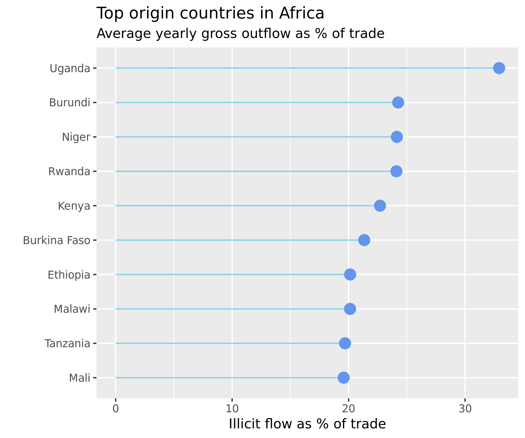
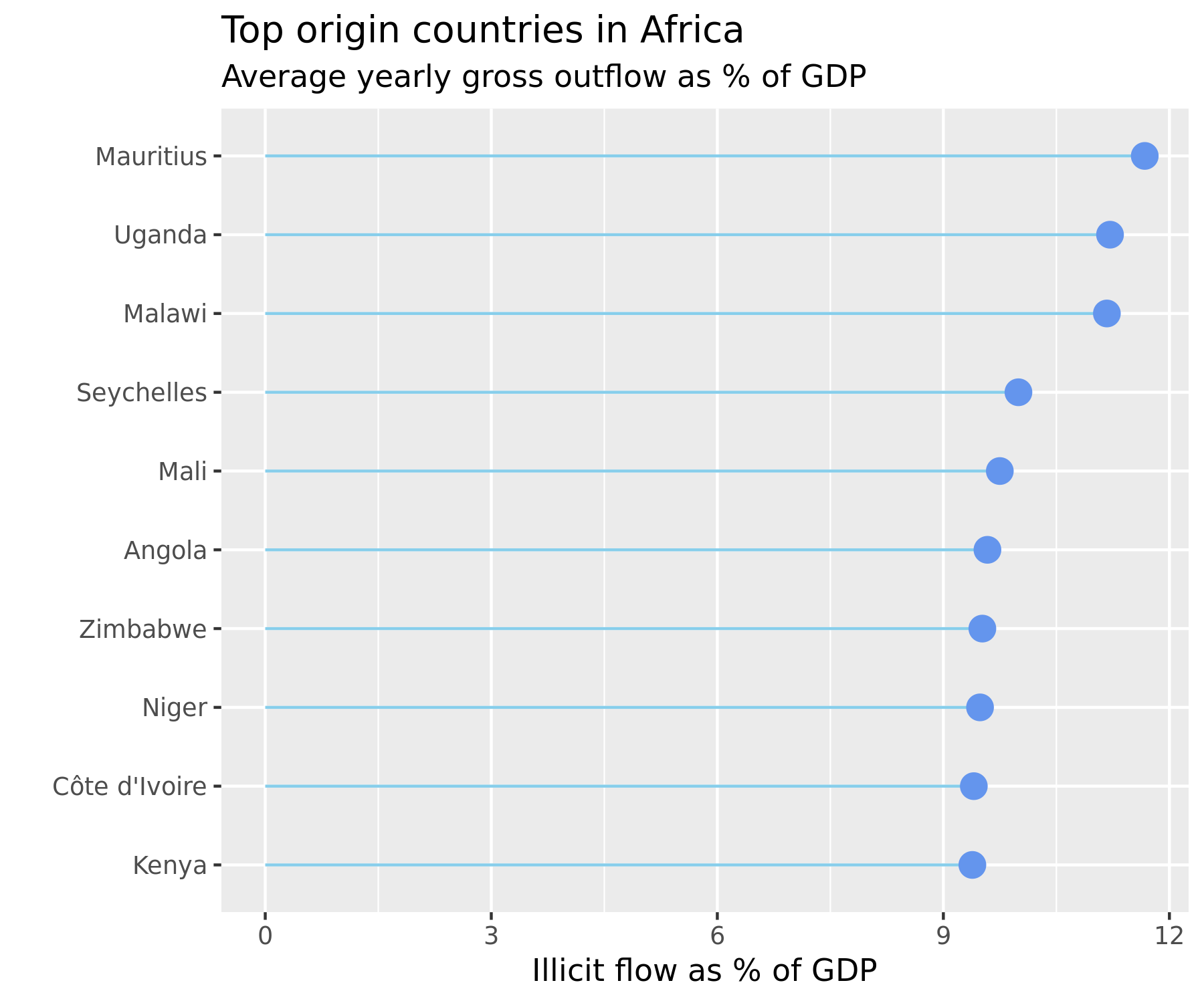
The interpretation should be carried out cautiously. The top loadings on the first principal components are Uganda, followed by Burkina Faso and Cameroon. Within Africa, Uganda is the country which experienced the highest gross outflows as a proportion of its total trade over the period 2000-2016, and the second highest as a proportion of its GDP over that same period (see figure below).
 Source: generated by
 Data Visualization.R in https://github.com/walice/Trade-IFF)
 Source: generated by
 Data Visualization.R in https://github.com/walice/Trade-IFF)
It is interesting to note that the PCA algorithm does not identify the countries which had the highest average dollar value of illicit outflows during 2000-2016, which were South Africa and Angola. This is because the data has been standardized to have mean 0 and unit variance, as is common when conducting PCA, since PCA is sensitive to outliers.
Rather, the PCA algorithm recovers in the top loadings for the most important principal components many of the countries that were among the top origins for outflows relative to trade or GDP, such as Burkina Faso, Ethiopia, Malawi, Seychelles, Mali, and Zimbabwe, even though the algorithm was run on (standardized) dollar values of outflows.
Explained variance
The first 6 principal components explain 63% of the variance in the data, with the first principal component explaining 38% of the variance alone.
scree_plot(country_features, show_explained_var=True)
| PC | var | |
|---|---|---|
| 0 | 1 | 3.763510e-01 |
| 1 | 2 | 7.215794e-02 |
| 2 | 3 | 5.939846e-02 |
| 3 | 4 | 5.123519e-02 |
| 4 | 5 | 3.787572e-02 |
| 5 | 6 | 3.396778e-02 |
| 6 | 7 | 3.106831e-02 |
| 7 | 8 | 2.638919e-02 |
| 8 | 9 | 2.585997e-02 |
| 9 | 10 | 2.268292e-02 |
| 10 | 11 | 2.200332e-02 |
| 11 | 12 | 2.037173e-02 |
| 12 | 13 | 1.925219e-02 |
| 13 | 14 | 1.910017e-02 |
| 14 | 15 | 1.719724e-02 |
| 15 | 16 | 1.561816e-02 |
| 16 | 17 | 1.346239e-02 |
| 17 | 18 | 1.260948e-02 |
| 18 | 19 | 1.150043e-02 |
| 19 | 20 | 1.118470e-02 |
| 20 | 21 | 1.060775e-02 |
| 21 | 22 | 8.985424e-03 |
| 22 | 23 | 8.762526e-03 |
| 23 | 24 | 8.330893e-03 |
| 24 | 25 | 6.857884e-03 |
| 25 | 26 | 6.636890e-03 |
| 26 | 27 | 5.660594e-03 |
| 27 | 28 | 5.216669e-03 |
| 28 | 29 | 4.582342e-03 |
| 29 | 30 | 4.137391e-03 |
| 30 | 31 | 3.673426e-03 |
| 31 | 32 | 3.514407e-03 |
| 32 | 33 | 3.274164e-03 |
| 33 | 34 | 3.004834e-03 |
| 34 | 35 | 2.840875e-03 |
| 35 | 36 | 2.611974e-03 |
| 36 | 37 | 2.263592e-03 |
| 37 | 38 | 2.120142e-03 |
| 38 | 39 | 1.688935e-03 |
| 39 | 40 | 1.536694e-03 |
| 40 | 41 | 1.461075e-03 |
| 41 | 42 | 1.319987e-03 |
| 42 | 43 | 9.527948e-04 |
| 43 | 44 | 6.724485e-04 |
| 44 | 45 | 1.776402e-33 |
| 45 | 46 | 1.776402e-33 |
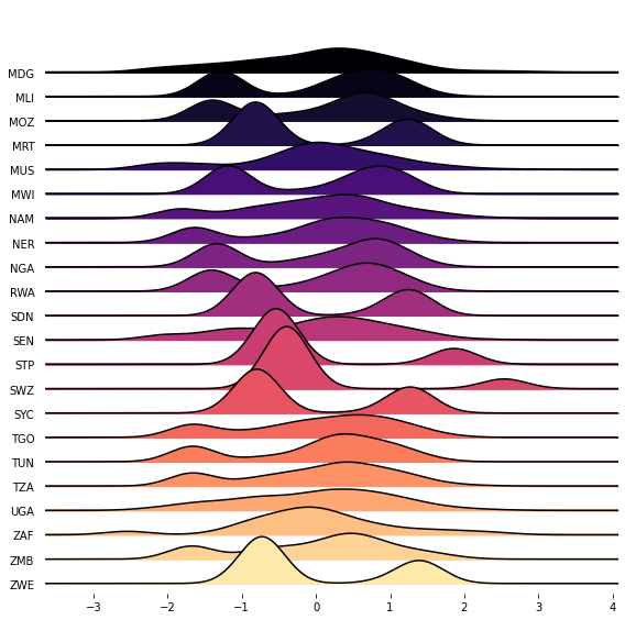
Variance-stabilizing and normalizing transformations
The figures below display the distribution of the mis-invoiced trade in each of the features of the feature space (after dropping those countries with 0 outflows in all sectors).
# Figure out which columns are composed of all 0s
country_features.apply(lambda x: (x == 0).all(), axis=0)
reporter.ISO
AGO False
BDI False
BEN False
BFA False
BWA False
CAF False
CIV False
CMR False
COG False
COM False
CPV False
DZA False
EGY False
ETH False
GAB False
GHA False
GIN False
GMB False
GNB False
KEN False
LBY True
LSO False
MAR False
MDG False
MLI False
MOZ False
MRT False
MUS False
MWI False
NAM False
NER False
NGA False
RWA False
SDN False
SEN False
SLE True
STP False
SWZ False
SYC False
TGO False
TUN False
TZA False
UGA False
ZAF False
ZMB False
ZWE False
dtype: bool
# Drop the corresponding features
country_features = country_features.drop(columns=['LBY', 'SLE'])
Again, I explore the consequences of applying a modified log transformation and a Yeo-Johnson transformation, respectively.
country_features_log = country_features.apply(lambda x: np.log(x+1) if np.issubdtype(x.dtype, np.number) else x, axis=0)
country_features_yeo = power_transform(country_features, method='yeo-johnson', standardize=True)
The top loadings on the first principal component, in both transformations, capture an origin hub located in the north-west of the continent with Benin, Niger, and Senegal featuring heavily.
The top loadings on the second principal component capture a south-southeast axis which runs from Gabon to Angola to Swaziland (now called Eswatini).
biplot_PCA(country_features_log, 10, 1, 2, obs='section')
biplot_PCA(country_features_yeo, 10, 1, 2, obs='section')
PCA on bilateral trade matrix
The previous sections explored relevant dimensions of variation by considering the feature space spanned by the origin of the illicit outflows, whether it be the source countries or the source sectors.
Now, I turn to exploring the relevant dimensions of illicit flows by analyzing the feature space spanned by the destination of those illicit outflows.
Let’s apply the create_features() function to the summary data-set IFF_Dest, where we have \(p=167\).
partner_features = create_features(IFF_Dest_Imp, 'Imp_IFF_hi',
features='partner.ISO', obs='reporter.ISO')
partner_features
| partner.ISO | AGO | ALB | AND | ARE | ARG | ARM | ATG | AUS | AUT | AZE | ... | URY | USA | VCT | VEN | VNM | VUT | YEM | ZAF | ZMB | ZWE | |
|---|---|---|---|---|---|---|---|---|---|---|---|---|---|---|---|---|---|---|---|---|---|---|
| reporter.ISO | year | |||||||||||||||||||||
| AGO | 2009 | 0.0 | 0.0 | 0.0 | 0.000000e+00 | 6.014820e+07 | 0.0 | 0 | 6.980492e+06 | 3.119279e+05 | 0.000000 | ... | 2.361993e+06 | 9.270820e+08 | 0 | 0.0 | 4.734647e+07 | 0 | 0.000000 | 1.016827e+09 | 1.060946e+05 | 309894.487818 |
| 2010 | 0.0 | 0.0 | 0.0 | 0.000000e+00 | 2.963158e+07 | 0.0 | 0 | 2.971282e+06 | 5.626929e+06 | 18935.636990 | ... | 1.644130e+06 | 8.268511e+08 | 0 | 0.0 | 2.970677e+07 | 0 | 0.000000 | 3.315930e+08 | 2.665205e+04 | 420951.156359 | |
| 2011 | 0.0 | 0.0 | 0.0 | 0.000000e+00 | 5.044258e+07 | 0.0 | 0 | 9.077825e+06 | 2.409418e+06 | 20266.842796 | ... | 1.016561e+06 | 8.601995e+08 | 0 | 0.0 | 2.451965e+07 | 0 | 0.000000 | 3.281534e+08 | 4.525653e+05 | 0.000000 | |
| 2012 | 0.0 | 0.0 | 0.0 | 0.000000e+00 | 2.055669e+08 | 0.0 | 0 | 7.483480e+06 | 1.354856e+07 | 22457.788787 | ... | 1.582490e+06 | 1.441162e+09 | 0 | 0.0 | 5.942382e+07 | 0 | 354866.063494 | 7.944924e+08 | 1.180964e+03 | 0.000000 | |
| 2013 | 0.0 | 0.0 | 0.0 | 0.000000e+00 | 5.839522e+07 | 0.0 | 0 | 1.569576e+07 | 8.770795e+06 | 1734.698687 | ... | 3.447835e+06 | 7.139003e+08 | 0 | 0.0 | 3.931132e+07 | 0 | 0.000000 | 4.272753e+08 | 2.855892e+05 | 0.000000 | |
| ... | ... | ... | ... | ... | ... | ... | ... | ... | ... | ... | ... | ... | ... | ... | ... | ... | ... | ... | ... | ... | ... | ... |
| ZWE | 2011 | 0.0 | 0.0 | 0.0 | 5.290029e+07 | 2.310119e+07 | 0.0 | 0 | 2.325259e+06 | 3.171896e+05 | 0.000000 | ... | 2.721346e+04 | 6.462989e+08 | 0 | 0.0 | 5.288219e+06 | 0 | 0.000000 | 3.088036e+09 | 5.016118e+07 | 0.000000 |
| 2012 | 0.0 | 0.0 | 0.0 | 5.923175e+07 | 1.011059e+07 | 0.0 | 0 | 1.664879e+06 | 1.220841e+06 | 0.000000 | ... | 0.000000e+00 | 6.069423e+08 | 0 | 0.0 | 4.745996e+06 | 0 | 0.000000 | 1.242790e+09 | 1.704507e+08 | 0.000000 | |
| 2013 | 0.0 | 0.0 | 0.0 | 0.000000e+00 | 0.000000e+00 | 0.0 | 0 | 0.000000e+00 | 0.000000e+00 | 0.000000 | ... | 0.000000e+00 | 0.000000e+00 | 0 | 0.0 | 0.000000e+00 | 0 | 0.000000 | 0.000000e+00 | 0.000000e+00 | 0.000000 | |
| 2014 | 0.0 | 0.0 | 0.0 | 0.000000e+00 | 0.000000e+00 | 0.0 | 0 | 0.000000e+00 | 0.000000e+00 | 0.000000 | ... | 0.000000e+00 | 0.000000e+00 | 0 | 0.0 | 0.000000e+00 | 0 | 0.000000 | 0.000000e+00 | 0.000000e+00 | 0.000000 | |
| 2015 | 0.0 | 0.0 | 0.0 | 5.042948e+07 | 0.000000e+00 | 0.0 | 0 | 5.764013e+05 | 6.721992e+05 | 0.000000 | ... | 9.012925e+04 | 4.109564e+07 | 0 | 0.0 | 3.093477e+03 | 0 | 0.000000 | 6.474374e+08 | 0.000000e+00 | 0.000000 |
624 rows × 167 columns
Biplots
The figure below displays the first and second principal components. It appears that the first principal component recovers the top destinations of illicit outflows, as the first loading corresponds to China which was the top average destination for illicit outflows from Africa during 2000-2016, and the second loading corresponds to the United States which was the second largest destination.
biplot_PCA(partner_features, 10, 1, 2, show_loadings=True)
| PC1 | PC2 | PC3 | PC4 | PC5 | PC6 | PC7 | PC8 | PC9 | PC10 | |
|---|---|---|---|---|---|---|---|---|---|---|
| AGO | 0.064538 | -0.127775 | -0.044675 | -0.081190 | 0.015199 | -0.030508 | -0.020684 | -0.075254 | 0.026087 | 0.018444 |
| ALB | 0.044858 | 0.100240 | -0.085332 | 0.010378 | 0.222166 | -0.056160 | 0.016405 | -0.068677 | 0.098802 | -0.006931 |
| AND | 0.002434 | 0.006593 | -0.006567 | 0.005445 | -0.015707 | 0.021064 | -0.006253 | -0.004508 | 0.001468 | -0.016877 |
| ARE | 0.091433 | -0.038099 | 0.067933 | -0.046062 | 0.123878 | -0.061712 | -0.030800 | 0.190913 | -0.147428 | 0.060691 |
| ARG | 0.129513 | 0.139207 | -0.082968 | 0.019367 | -0.043149 | 0.085106 | -0.014389 | 0.038525 | 0.024086 | 0.000942 |
| ... | ... | ... | ... | ... | ... | ... | ... | ... | ... | ... |
| VUT | 0.000000 | 0.000000 | 0.000000 | 0.000000 | -0.000000 | 0.000000 | 0.000000 | 0.000000 | 0.000000 | 0.000000 |
| YEM | 0.040005 | -0.060918 | 0.007451 | 0.143530 | 0.037673 | 0.037506 | 0.085598 | 0.261330 | 0.309931 | -0.017295 |
| ZAF | 0.008847 | 0.007834 | 0.091261 | -0.022447 | 0.026785 | 0.001632 | -0.043753 | 0.104236 | -0.037778 | 0.124183 |
| ZMB | 0.040152 | 0.020620 | -0.037492 | 0.009481 | 0.093282 | -0.176393 | -0.033166 | 0.069316 | -0.109787 | 0.018559 |
| ZWE | 0.058102 | -0.112442 | 0.020694 | 0.215291 | 0.042842 | 0.010566 | 0.044425 | 0.149634 | 0.182897 | 0.017658 |
167 rows × 10 columns
 Source: generated by
 Data Visualization.R in https://github.com/walice/Trade-IFF
The top loadings on the other principal components reveal some unexpected sources of variation for destination countries.
The top loadings are:
Second principal component:
Top loading 1: El Salvador
Top loading 2: Dominican Republic
Top loading 3: Nepal
Third principal component:
Top loading 1: Belgium
Top loading 2: Norway
Top loading 3: Panama
Fourth principal component:
Top loading 1: Iran
Top loading 2: Suriname
Top loading 3: Papua New Guinea
Fifth principal component:
Top loading 1: Central African Republic
Top loading 2: Kuwait
Top loading 3: Albania
Sixth principal component:
Top loading 1: Ecuador
Top loading 2: Slovenia
Top loading 3: Algeria
These dimensions of variation are much harder to interpret. Nevertheless, a few points stand out.
First, apart from the first principal component, the loadings do not appear to be driven by the magnitude of the illicit outflows. Second, the loadings recovered are surprising. One “usual suspect” which appears is Panama (on the third principal component) which is one of the oldest and best-known tax haven in the Americas. Third, this suggests that the analysis of the destinations of illicit outflows from Africa merits much deeper analysis to “follow the money” (which is outside the scope of this project).
biplot_PCA(partner_features, 10, 3, 4)
biplot_PCA(partner_features, 10, 5, 6)
Explained variance
With a feature space of \(p=167\), 12 principal components are required to explain at least 50% of the variance in the data.
scree_plot(partner_features)
Variance-stabilizing and normalizing transformations
The sections below explore the effect of variance-stabilizing transformations on the partner_features data-set.
Korea and Nicaragua appear as top loadings on the first and second principal components, respectively.
When running PCA on the transformed data, the projection of the principal component scores on the first two principal components takes on a half-moon shape.
Expand the code chunks to see the details.
# Figure out which columns are composed of all 0s
partner_features.apply(lambda x: (x == 0).all(), axis=0)
noIFFpartner = partner_features.loc[:,partner_features.apply(lambda x: (x == 0).all(), axis=0)].columns.tolist()
noIFFpartner
['ATG',
'BLZ',
'BMU',
'DMA',
'GNB',
'GRD',
'KGZ',
'KNA',
'LCA',
'SLB',
'TON',
'VCT',
'VUT']
# Drop the corresponding features
partner_features = partner_features.drop(columns=noIFFpartner)
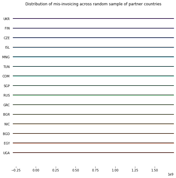
# Plot the distribution of illicit flows for a random sample of partner countries
fig, axes = joypy.joyplot(partner_features.sample(n=15, axis=1, random_state=234),
colormap=plt.cm.rainbow, figsize=(8,8),
title='Distribution of mis-invoicing across random sample of partner countries');
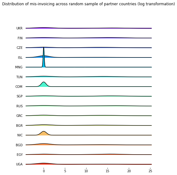
# Apply a modified log transformation
partner_features_log = partner_features.apply(lambda x: np.log(x+1) if np.issubdtype(x.dtype, np.number) else x, axis=1)
# Plot the distribution of illicit flows for the transformed data
fig, axes = joypy.joyplot(partner_features_log.sample(n=15, axis=1, random_state=234),
colormap=plt.cm.rainbow, figsize=(8,8),
title='Distribution of mis-invoicing across random sample of partner countries (log transformation)');
# Biplot for the first 2 principal components for the transformed data (modified log)
biplot_PCA(partner_features_log, 10, 1, 2)
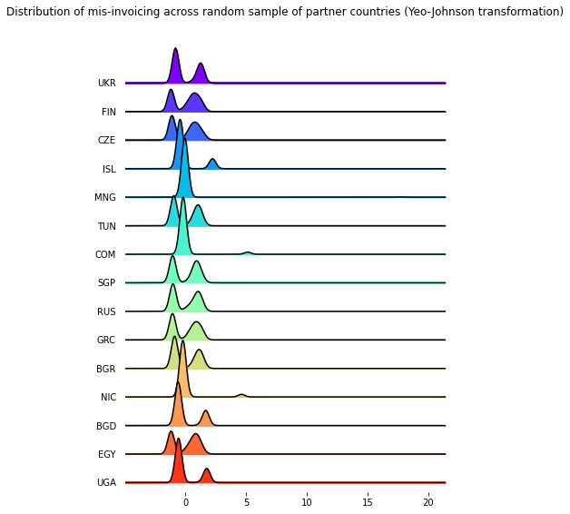
# Apply a modified Yeo-Johnson transformation
partner_features_yeo = power_transform(partner_features, method='yeo-johnson', standardize=True)
# Plot the distribution of illicit flows for the transformed data
partner_features_yeo = pd.DataFrame(partner_features_yeo,
index=partner_features.index,
columns=partner_features.columns)
random.seed(234)
fig, axes = joypy.joyplot(partner_features_yeo.sample(n=15, axis=1, random_state=234),
colormap=plt.cm.rainbow, figsize=(8,8),
title='Distribution of mis-invoicing across random sample of partner countries (Yeo-Johnson transformation)');
# Biplot for the first 2 principal components for the transformed data (Yeo-Johnson)
biplot_PCA(partner_features_yeo, 10, 1, 2)
Intra-African illicit financial flows
The analysis will now be restricted to intra-African illicit financial flows, that is, illicit capital that originates from African countries and which flows to African countries too.
Data wrangling
# Import bilateral trade mis-invoicing data
IFF_Dest = pd.read_csv('Data/GER_Orig_Dest_Year_Africa.csv')
# Restrict to destinations in Africa only
IFF_Dest_AFR = IFF_Dest[IFF_Dest['pRegion'] == 'Africa']
IFF_Dest_AFR = IFF_Dest_AFR.fillna(0).drop(columns=['reporter', 'rIncome', 'rDev',
'partner', 'pRegion', 'pIncome', 'pDev',
'Imp_IFF_lo', 'Exp_IFF_lo']) \
.set_index(['reporter.ISO', 'year'])
# Extract trade mis-invoicing in imports and exports, respectively
IFF_Dest_Imp_AFR = IFF_Dest_AFR[['partner.ISO', 'Imp_IFF_hi']]
IFF_Dest_Exp_AFR = IFF_Dest_AFR[['partner.ISO', 'Exp_IFF_hi']]
Let’s create the feature space from the African partner countries which are the destinations of illicit ouflows originating from the countries listed in reporter.ISO.
partner_features_AFR = create_features(IFF_Dest_Imp_AFR, 'Imp_IFF_hi',
features='partner.ISO', obs='reporter.ISO')
partner_features_AFR
| partner.ISO | AGO | BDI | BEN | BFA | BWA | CAF | CIV | CMR | COG | COM | ... | STP | SWZ | SYC | TGO | TUN | TZA | UGA | ZAF | ZMB | ZWE | |
|---|---|---|---|---|---|---|---|---|---|---|---|---|---|---|---|---|---|---|---|---|---|---|
| reporter.ISO | year | |||||||||||||||||||||
| AGO | 2009 | 0.0 | 0.0 | 0.0 | 0.0 | 0.000000e+00 | 0.0 | 7.356525e+05 | 0.000000 | 0.000000e+00 | 0.0 | ... | 0.000000 | 0.0 | 0.0 | 0.000000 | 1.628157e+06 | 0.000000e+00 | 0.0 | 1.016827e+09 | 1.060946e+05 | 309894.487818 |
| 2010 | 0.0 | 0.0 | 0.0 | 0.0 | 2.025235e+05 | 0.0 | 5.577699e+07 | 53088.378146 | 1.402793e+08 | 0.0 | ... | 0.000000 | 0.0 | 0.0 | 252999.300576 | 1.137066e+08 | 5.529461e+03 | 0.0 | 3.315930e+08 | 2.665205e+04 | 420951.156359 | |
| 2011 | 0.0 | 0.0 | 0.0 | 0.0 | 5.501246e+03 | 0.0 | 6.262938e+06 | 257786.746458 | 3.466061e+07 | 0.0 | ... | 0.000000 | 0.0 | 0.0 | 0.000000 | 4.623718e+07 | 1.745372e+06 | 0.0 | 3.281534e+08 | 4.525653e+05 | 0.000000 | |
| 2012 | 0.0 | 0.0 | 0.0 | 0.0 | 0.000000e+00 | 0.0 | 1.425377e+07 | 222663.224270 | 2.587614e+07 | 0.0 | ... | 8435.069683 | 0.0 | 0.0 | 0.000000 | 1.262796e+07 | 1.253616e+05 | 0.0 | 7.944924e+08 | 1.180964e+03 | 0.000000 | |
| 2013 | 0.0 | 0.0 | 0.0 | 0.0 | 2.945193e+05 | 0.0 | 2.125395e+06 | 0.000000 | 4.357466e+06 | 0.0 | ... | 957.605075 | 0.0 | 0.0 | 0.000000 | 4.438123e+06 | 1.035603e+05 | 0.0 | 4.272753e+08 | 2.855892e+05 | 0.000000 | |
| ... | ... | ... | ... | ... | ... | ... | ... | ... | ... | ... | ... | ... | ... | ... | ... | ... | ... | ... | ... | ... | ... | ... |
| ZWE | 2011 | 0.0 | 0.0 | 0.0 | 0.0 | 8.741233e+07 | 0.0 | 0.000000e+00 | 0.000000 | 0.000000e+00 | 0.0 | ... | 0.000000 | 0.0 | 0.0 | 0.000000 | 0.000000e+00 | 1.295280e+06 | 0.0 | 3.088036e+09 | 5.016118e+07 | 0.000000 |
| 2012 | 0.0 | 0.0 | 0.0 | 0.0 | 3.187848e+07 | 0.0 | 0.000000e+00 | 0.000000 | 0.000000e+00 | 0.0 | ... | 0.000000 | 0.0 | 0.0 | 0.000000 | 0.000000e+00 | 2.729399e+06 | 0.0 | 1.242790e+09 | 1.704507e+08 | 0.000000 | |
| 2013 | 0.0 | 0.0 | 0.0 | 0.0 | 0.000000e+00 | 0.0 | 0.000000e+00 | 0.000000 | 0.000000e+00 | 0.0 | ... | 0.000000 | 0.0 | 0.0 | 0.000000 | 0.000000e+00 | 0.000000e+00 | 0.0 | 0.000000e+00 | 0.000000e+00 | 0.000000 | |
| 2014 | 0.0 | 0.0 | 0.0 | 0.0 | 0.000000e+00 | 0.0 | 0.000000e+00 | 0.000000 | 0.000000e+00 | 0.0 | ... | 0.000000 | 0.0 | 0.0 | 0.000000 | 0.000000e+00 | 0.000000e+00 | 0.0 | 0.000000e+00 | 0.000000e+00 | 0.000000 | |
| 2015 | 0.0 | 0.0 | 0.0 | 0.0 | 8.142369e+06 | 0.0 | 0.000000e+00 | 0.000000 | 0.000000e+00 | 0.0 | ... | 0.000000 | 0.0 | 0.0 | 0.000000 | 0.000000e+00 | 8.238550e+06 | 0.0 | 6.474374e+08 | 0.000000e+00 | 0.000000 |
604 rows × 46 columns
There are strong regional dynamics in international trade, so it is useful to extract information on which regions the countries belong to. The crosswalk data-set includes information on the geographical groupings of each country. The codes are taken from the UN Statistics Division M49 standard (https://unstats.un.org/unsd/methodology/m49/).
The UN_Intermediate_Region code is nested within the UN_Sub-region code. In the M49 standard grouping for Africa, there are two sub-regions: Northern Africa and Sub-Saharan Africa. The latter contains further geographical groupings: Eastern Africa, Middle Africa, Southern Africa, Western Africa. Therefore, we need to reconcile both so that the regional labels include Northern Africa and the 4 groupings within Sub-Saharan Africa. The code below achieves this, and this is automatized by the region_labels() function further down.
# Merge in UN Intermediate Region groups
partner_features_AFR = pd.merge(left=partner_features_AFR.reset_index(),
right=crosswalk[['ISO3166.3', 'UN_Intermediate_Region']].drop_duplicates('ISO3166.3'),
how='left',
left_on='reporter.ISO', right_on='ISO3166.3')
# Which African countries do not have a UN Intermediate region?
noregion_mask = partner_features_AFR['UN_Intermediate_Region'].isnull()
countries_noregion = partner_features_AFR[noregion_mask]['reporter.ISO'].unique().tolist()
countries_noregion
['DZA', 'EGY', 'LBY', 'MAR', 'SDN', 'TUN']
# Which UN Sub-region do those countries belong to?
crosswalk[crosswalk['ISO3166.3'].isin(countries_noregion)]['UN_Sub-region'].unique()
array(['Northern Africa'], dtype=object)
# Assign Northern Africa as a group for those countries
partner_features_AFR.loc[partner_features_AFR['reporter.ISO'].isin(countries_noregion), 'UN_Intermediate_Region'] = 'Northern Africa'
partner_features_AFR = partner_features_AFR.set_index(['reporter.ISO', 'year']).drop(columns=['ISO3166.3', 'UN_Intermediate_Region'])
The figure below displays the biplot for the first two principal components estimated using the intra-African bilateral matrix of illicit flows.
biplot_PCA(partner_features_AFR, partner_features_AFR.shape[1], 1, 2)
The countries with the top 3 loadings on the first principal component are Mozambique (MOZ), Madagascar (MDG) and Comoros (COM). Madagascar and the Comoros are islands in the Mozambique channel, where two well-known conduits of illicit financial flows are located: the Seychelles and Mauritius.
The second principal component seems to capture Northern Africa, with Algeria and Tunisia scoring the second and third largest loading, respectively.
Removing outliers
There are vibrant debates in the field on estimating trade mis-invoicing based on mismatches in official trade data, much of which is outside the scope of this project. However, suffice to say that there are some outliers that might have large values of mis-invoicing due to benign reasons. For example, South Africa does not report gold exports to UN Comtrade (the underlying source of official trade statistis), and so any discrepancies found by looking at its mirrored trade statistics would result in spurious mis-invoicing estimates.
I remove outliers based on extreme values on the first two principal components. This effectively removes most of the observations for South Africa. Further work is needed, though, to remove outliers based on domain knowledge, especially if using this data to do a deep dive on certain dimensions (rather than looking at aggregate patterns, as is the case here).
features_data_std = StandardScaler().fit_transform(partner_features_AFR)
pca = PCA(n_components=partner_features_AFR.shape[1])
princ_comp = pca.fit_transform(features_data_std)
outlying = (princ_comp[:,0] > 6) | (princ_comp[:,1] > 4)
partner_features_AFR[outlying].index
MultiIndex([('AGO', 2010),
('CIV', 2013),
('EGY', 2012),
('GHA', 2002),
('MAR', 2005),
('MAR', 2006),
('MAR', 2007),
('MAR', 2008),
('MAR', 2009),
('MAR', 2010),
('MAR', 2011),
('MAR', 2012),
('NGA', 2011),
('ZAF', 2005),
('ZAF', 2006),
('ZAF', 2008),
('ZAF', 2010),
('ZAF', 2011),
('ZAF', 2012),
('ZAF', 2013),
('ZAF', 2014),
('ZAF', 2015),
('ZAF', 2016)],
names=['reporter.ISO', 'year'])
partner_features_AFR_noout = partner_features_AFR[~outlying]
The figure below displays the projection of the data without outliers on the first 2 principal components. Some interesting regional patterns appear.
Top loadings on the first principal component seem to capture a western African hub, with Cote d’Ivoire and Togo scoring highly. By contrast, the second principal component seems to recover a southern African hub, with top loadings going to South Africa, Malawi, and Botswana.
biplot_PCA(partner_features_AFR_noout, 46, 1, 2)
In order to discern better any groupings, the next section will color the observations according to an aggregate class label.
Coloring by class label
The function region_labels() extracts the regional labels from the crosswalk and further divides the “Sub-Saharan Africa” group into its 4 corresponding subgroups, as discussed above.
def region_labels(features_data):
"""
Return regional labels for countries in the data
features_data: as Pandas dataframe, data-set of features
"""
# Extract observation labels from features data
obs_labels = pd.DataFrame(features_data.reset_index().set_index('reporter.ISO').index)
# Merge with UN intermediate regions from crosswalk
obs_labels = pd.merge(left=obs_labels,
right=crosswalk[['ISO3166.3', 'UN_Intermediate_Region']].drop_duplicates('ISO3166.3'),
how='left',
left_on='reporter.ISO', right_on='ISO3166.3') \
.drop(columns='ISO3166.3')
# Create a mask for the Northern African regions and replace the missing intermediate region
noregion_mask = obs_labels['UN_Intermediate_Region'].isnull()
countries_noregion = obs_labels[noregion_mask]['reporter.ISO'].unique().tolist()
obs_labels.loc[obs_labels['reporter.ISO'].isin(countries_noregion), 'UN_Intermediate_Region'] = 'Northern Africa'
return obs_labels
The function biplot_PCA_classes() projects the data in the two principal components chosen by the user, and further colors the observations either according to their UN regional grouping (by specifying classes='UN_Intermediate_Region') or according to their World Bank income group classification (by specifying classes='Income group (World Bank)').
def biplot_PCA_classes(features_data, nPC=2, firstPC=1, secondPC=2, classes='UN_Intermediate_Region'):
"""
Projects the data in the 2-dimensional space spanned by 2 principal components
chosen by the user, along with a bi-plot of the top 3 loadings per PC, and colors
by class label.
Args:
features_data: data-set of features
nPC: number of principal components
firstPC: integer denoting first principal component to plot in bi-plot
secondPC: integer denoting second principal component to plot in bi-plot
classes: {'UN_Intermediate_Region', 'Income group (World Bank)'}, as string, class label
by which to color observations
Returns:
plot (interactive)
pca_loadings (if show_loadings=True)
"""
# Unit of observation is the reporting country
obs='reporter.ISO'
# Run PCA (standardize beforehand)
features_data_std = StandardScaler().fit_transform(features_data)
# features_data_std = power_transform(features_data, method='yeo-johnson', standardize=True)
pca = PCA(n_components=nPC, random_state=234)
princ_comp = pca.fit_transform(features_data_std)
# Loadings
cols = ['PC' + str(c+1) for c in np.arange(nPC)]
pca_loadings = pd.DataFrame(pca.components_.T,
columns=cols,
index=list(features_data.columns))
# Scores
pca_scores = pd.DataFrame(princ_comp,
columns=cols)
pca_scores[obs] = features_data.reset_index()[obs].values.tolist()
pca_scores['year'] = features_data.reset_index()['year'].values.tolist()
score_PC1 = princ_comp[:,firstPC-1]
score_PC2 = princ_comp[:,secondPC-1]
# Plot data
plot_data = pd.merge(pca_scores, obs_info, on=[obs, 'year'])
tooltip_obs = ['reporter', 'year', 'Income group (World Bank)', 'Country status (UN)']
obs_labels = region_labels(features_data)
plot_data = pd.merge(left=plot_data, right=obs_labels.drop_duplicates('reporter.ISO'), on='reporter.ISO')
if classes == 'UN_Intermediate_Region':
color_scheme = 'paired'
else:
color_scheme = 'dark2'
# Return chosen PCs to plot
PC1 = 'PC'+str(firstPC)
PC2 = 'PC'+str(secondPC)
# Top loadings (in absolute value)
# TO DO: use dict to iterate over
toploadings_PC1 = pca_loadings.apply(lambda x: abs(x)).sort_values(by=PC1).tail(3)[[PC1, PC2]]
toploadings_PC2 = pca_loadings.apply(lambda x: abs(x)).sort_values(by=PC2).tail(3)[[PC1, PC2]]
originsPC1 = pd.DataFrame({'index':toploadings_PC1.index.tolist(),
PC1: np.zeros(3),
PC2: np.zeros(3)})
originsPC2 = pd.DataFrame({'index':toploadings_PC2.index.tolist(),
PC1: np.zeros(3),
PC2: np.zeros(3)})
toploadings_PC1 = pd.concat([toploadings_PC1.reset_index(), originsPC1], axis=0)
toploadings_PC2 = pd.concat([toploadings_PC2.reset_index(), originsPC2], axis=0)
toploadings_PC1[PC1] = toploadings_PC1[PC1]*max(score_PC1)*1.5
toploadings_PC1[PC2] = toploadings_PC1[PC2]*max(score_PC2)*1.5
toploadings_PC2[PC1] = toploadings_PC2[PC1]*max(score_PC1)*1.5
toploadings_PC2[PC2] = toploadings_PC2[PC2]*max(score_PC2)*1.5
# Project top 3 loadings over the space spanned by 2 principal components
lines = alt.Chart().mark_line().encode()
for color, i, dataset in zip(['#440154FF', '#21908CFF'], [0,1], [toploadings_PC1, toploadings_PC2]):
lines[i] = alt.Chart(dataset).mark_line(color=color).encode(
x= PC1 +':Q',
y= PC2 +':Q',
detail='index'
).properties(
width=400,
height=400
)
# Add labels to the loadings
text=alt.Chart().mark_text().encode()
for color, i, dataset in zip(['#440154FF', '#21908CFF'], [0, 1], [toploadings_PC1[0:3], toploadings_PC2[0:3]]):
text[i] = alt.Chart(dataset).mark_text(
align='left',
baseline='bottom',
color=color
).encode(
x= PC1 +':Q',
y= PC2 +':Q',
text='index'
)
# Scatter plot colored by observation class label
points = alt.Chart(plot_data).mark_circle(size=60).encode(
x=alt.X(PC1, axis=alt.Axis(title='Principal Component ' + str(firstPC))),
y=alt.X(PC2, axis=alt.Axis(title='Principal Component ' + str(secondPC))),
color=alt.Color(classes, scale=alt.Scale(scheme=color_scheme),
legend=alt.Legend(orient='right')),
tooltip=tooltip_obs
).interactive()
chart = (points + lines[0] + lines[1] + text[0] + text[1])
chart.display()
The following graphs suggest that the first two components of PCA seem to partition the feature space remarkably well according to regional groupings, and to a lesser extent according to income grouping. It should be noted that there is less variation in the income groupings in Africa as a whole, with few countries belong to the high income group.
The biplot which uses African partner countries as the feature space (after removing outliers) and which colors by regional grouping is the most striking (scroll down below to see it). Recall that the loadings refer to the partner countries (i.e. the destinations of the illicit outflows) which have the heaviest loadings on the first/second principal components, while the observations are colored according to the reporter country (i.e. the origin of the illicit flow). This biplot suggests that the partner features which have the highest weight on the first principal components correspond to a western African hub (Cote d’Ivoire and Togo), and that those observations with the highest principal component scores in that rotated space correspond to western African reporting countries.
Similarly, the largest weights on the second principal component refer to a southern African partner hub (South Africa, Malawi, and Botswana), while the observations with the highest scores correspond to northern and southern African countries.
Therefore, it appears that there are strong sub-regional dynamics in intra-African illicit financial flows. The policy implication of this finding is that existing sub-regional policy initiatives could be leveraged to combat illicit financial flows within the continent. For example, the Economic Community of West African States (ECOWAS) could anchor policy efforts in western Africa while the East African Community (EAC) could attend to the east.
For sector features
biplot_PCA_classes(sector_features, 21, 1, 2, classes='UN_Intermediate_Region')
biplot_PCA_classes(sector_features, 21, 1, 2, classes='Income group (World Bank)')
For partner features
biplot_PCA_classes(partner_features, 46, 1, 2)
biplot_PCA_classes(partner_features, 46, 1, 2, classes='Income group (World Bank)')
For partner features, restricted to African partners
biplot_PCA_classes(partner_features_AFR, 46, 1, 2)
biplot_PCA_classes(partner_features_AFR, 46, 1, 2, classes='Income group (World Bank)')
For partner features, restricted to African partners, without outliers
biplot_PCA_classes(partner_features_AFR_noout, 46, 1, 2)
biplot_PCA_classes(partner_features_AFR_noout, 46, 1, 2, classes='Income group (World Bank)')
Clustering
Agglomerative clustering
This section investigates clustering techniques to see if they recover some of the groupings observed above.
# Run PCA on first 2 principal components on intra-African partners, without outliers
features_data_std = StandardScaler().fit_transform(partner_features_AFR_noout)
pca = PCA(n_components=10)
princ_comp = pca.fit_transform(features_data_std)
X = princ_comp[:,[0,1]]
# Perform agglomerative clustering
from sklearn.cluster import AgglomerativeClustering
clustering = AgglomerativeClustering(n_clusters=5, linkage='ward').fit(X)
plt.scatter(X[:, 0], X[:, 1], c=clustering.labels_);
plt.title('Agglomerative clustering using Ward linkage');
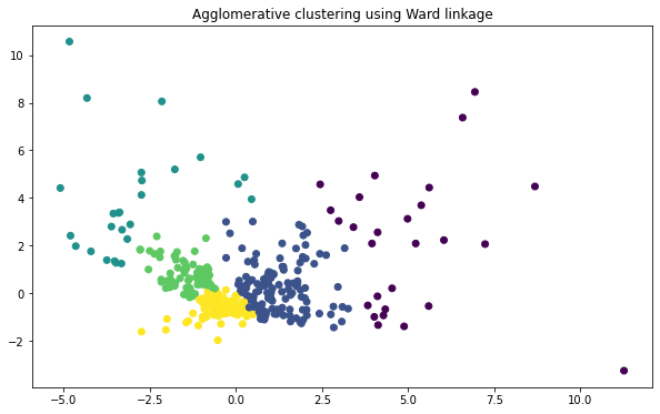
Agglomerative clustering with Ward linkage results in better identified clusters on the first two principal components (compared to single, complete, or average linkage; code omitted).
However, the groupings do not correspond to the ground truth labels of either region or income grouping. Let’s briefly investigate the observation labels in each cluster to see if discernable patterns appear. The labels in the first cluster are given by:
# Show labels in first cluster
partner_features_AFR_noout.index[np.where(clustering.labels_ == 0)[0]]
MultiIndex([('AGO', 2011),
('AGO', 2012),
('BEN', 2013),
('BEN', 2014),
('BFA', 2014),
('CIV', 2008),
('CIV', 2009),
('CIV', 2010),
('CIV', 2011),
('CIV', 2012),
('CIV', 2014),
('CMR', 2012),
('CMR', 2014),
('DZA', 2014),
('DZA', 2015),
('DZA', 2016),
('EGY', 2015),
('ETH', 2012),
('GHA', 2000),
('GHA', 2001),
('GHA', 2010),
('GHA', 2013),
('MLI', 2007),
('MLI', 2010),
('MLI', 2011),
('MLI', 2012),
('NGA', 2013)],
names=['reporter.ISO', 'year'])
Let’s extract the unique country labels per cluster.
# Countries in first cluster
cluster_labels = partner_features_AFR_noout.index[np.where(clustering.labels_ == 0)[0]].to_list()
country_labels = [i[0] for i in cluster_labels]
set(country_labels)
{'AGO', 'BEN', 'BFA', 'CIV', 'CMR', 'DZA', 'EGY', 'ETH', 'GHA', 'MLI', 'NGA'}
No immediately discernable pattern appears in the first cluster. This is the case for the remaining clusters too (code hidden).
# Countries in second cluster
cluster_labels = partner_features_AFR_noout.index[np.where(clustering.labels_ == 1)[0]].to_list()
country_labels = [i[0] for i in cluster_labels]
set(country_labels)
{'AGO',
'BEN',
'BFA',
'CIV',
'CMR',
'COG',
'DZA',
'EGY',
'ETH',
'GAB',
'GHA',
'GIN',
'GMB',
'MAR',
'MLI',
'MRT',
'NER',
'NGA',
'SDN',
'SEN',
'TGO',
'TUN',
'ZAF'}
# Countries in third cluster
cluster_labels = partner_features_AFR_noout.index[np.where(clustering.labels_ == 2)[0]].to_list()
country_labels = [i[0] for i in cluster_labels]
set(country_labels)
{'AGO',
'BDI',
'EGY',
'MWI',
'NGA',
'RWA',
'SDN',
'TZA',
'UGA',
'ZAF',
'ZMB',
'ZWE'}
# Countries in fourth cluster
cluster_labels = partner_features_AFR_noout.index[np.where(clustering.labels_ == 3)[0]].to_list()
country_labels = [i[0] for i in cluster_labels]
set(country_labels)
{'BDI',
'BWA',
'EGY',
'KEN',
'MDG',
'MOZ',
'MWI',
'NAM',
'RWA',
'TZA',
'UGA',
'ZAF',
'ZMB',
'ZWE'}
# Countries in fifth cluster
cluster_labels = partner_features_AFR_noout.index[np.where(clustering.labels_ == 4)[0]].to_list()
country_labels = [i[0] for i in cluster_labels]
set(country_labels)
{'BDI',
'BEN',
'BFA',
'BWA',
'CAF',
'CIV',
'CMR',
'COG',
'COM',
'CPV',
'DZA',
'EGY',
'ETH',
'GAB',
'GHA',
'GIN',
'GMB',
'GNB',
'KEN',
'LBY',
'LSO',
'MAR',
'MDG',
'MLI',
'MOZ',
'MRT',
'MUS',
'MWI',
'NAM',
'NER',
'NGA',
'RWA',
'SDN',
'SEN',
'SLE',
'STP',
'SWZ',
'SYC',
'TGO',
'TUN',
'TZA',
'UGA',
'ZAF',
'ZMB',
'ZWE'}
Hierarchical clustering and corresponding heatmap
Rather than specifying ex ante the number of clusters, I now perform hierarchical clustering, restricting myself to illicit trade in 2016. I have explored various transformations, scalings, and types of linkages. I find that a (modified) log transformation on standardized data (with mean 0 and unit variance) with Ward linkage (which minimizes the sum of squared differences within all clusters) performs rather well.
# Create data for African bilateral trade matrix in 2016
data = partner_features_AFR_noout.reset_index() \
.query('year == "2016"').drop(columns='year').set_index('reporter.ISO')
# Select the columns which have at least 1 non-zero row
data = data.loc[:,(data != 0).any(axis=0)]
# Log the data
data = data.apply(lambda x: np.log10(x+1) if np.issubdtype(x.dtype, np.number) else x, axis=0)
# Scale the data
scaler = StandardScaler()
# scaler = MinMaxScaler()
data_scaled = scaler.fit_transform(data)
data_scaled = pd.DataFrame(data_scaled, index=data.index, columns=data.columns)
# Extract region labels for the observations
obs_labels = region_labels(data).set_index('reporter.ISO')
# Extract unique regions
color_labels = obs_labels['UN_Intermediate_Region'].unique()
color_labels = np.sort(color_labels)
# List of RGB triplets for the region labels
rgb_values = sns.color_palette('Paired', 5)
# Map region labels to RGB triplet
color_map = dict(zip(color_labels, rgb_values))
region_color = pd.DataFrame(obs_labels)['UN_Intermediate_Region'].map(color_map)
The reporting countries are plotted in the rows of the heatmap below, while the partner countries (restricted to non-outlying African countries) are displayed in the columns. Dendograms for each dimension are displayed. In addition, the first column colors the observations according to their ground truth regional label.
On the origins dimension (i.e. reporters), the two highest-level clusters correspond broadly to western African (in pink) countries on the one hand, and eastern (in light blue) and middle African (in dark blue) countries on the other.
# Plot heatmap and corresponding dendograms
g = sns.clustermap(data_scaled,
method='ward',
cmap='bone_r',
row_colors=region_color,
);
g.fig.suptitle('Hierarchical clustering with Ward linkage', y=1);
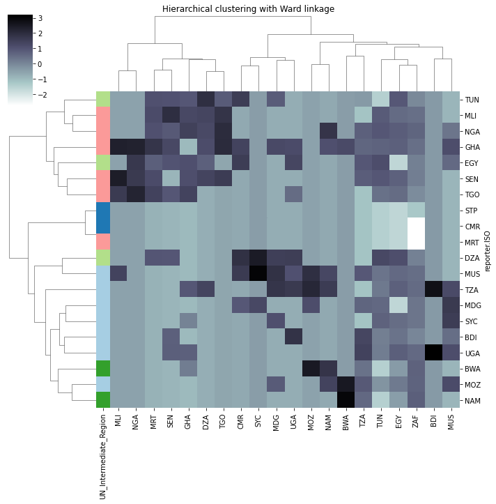
Network analysis
The matrix of bilateral mis-invoiced imports between African reporter countries and partner countries can be conceptualized as a weighted directed graph. Recall that the data-set IFF_Dest contains the mis-invoiced imports and exports for a reporter-partner-year tuple. The underlying data has been aggregated across commodity sectors using the Gross Excluding Reversals (GER) method, which ignores all inflows of capital (i.e. negative values), and simply sums up the positive outflows across trading partners.
The table below shows the IFF_Dest data-set that we are working with:
| reporter | reporter.ISO | rIncome | rDev | year | partner | partner.ISO | pRegion | pIncome | pDev | Imp_IFF_lo | Imp_IFF_hi | Exp_IFF_lo | Exp_IFF_hi | |
|---|---|---|---|---|---|---|---|---|---|---|---|---|---|---|
| 0 | Algeria | DZA | UMC | Developing | 2001 | Andorra | AND | Europe | HIC | Developed | 7.925637e+03 | 1.609561e+04 | NaN | NaN |
| 1 | Algeria | DZA | UMC | Developing | 2001 | Argentina | ARG | Americas | HIC | Developing | 1.914238e+07 | 4.717459e+07 | NaN | NaN |
| 2 | Algeria | DZA | UMC | Developing | 2001 | Australia | AUS | Oceania | HIC | Developed | 1.589172e+06 | 2.027641e+07 | NaN | 1412.374399 |
| 3 | Algeria | DZA | UMC | Developing | 2001 | Austria | AUT | Europe | HIC | Developed | 1.511117e+07 | 7.641706e+07 | NaN | NaN |
| 4 | Algeria | DZA | UMC | Developing | 2001 | Belgium | BEL | Europe | HIC | Developed | 9.357981e+06 | 2.285729e+07 | NaN | NaN |
Thus, the values in the import column of IFF_Dest correspond to import over-invoicing which result in an illicit outflow from reporter \(i\) to partner \(j\). Therefore, we can consider each entry in IFF_Dest to represent an edge going out from the reporter into the partner country.
Data wrangling
Let’s download some indicators from the World Bank that we can use as node attributes.
The covariates control-corruption and rule-of-law refer to the percentile rank that each country achieves on these governance dimensions. The control of corruption measure captures perceptions of the extent to which public power is exercised for private gain, including both petty and grand forms of corruption, as well as “capture” of the state by elites and private interests. The rule of law variable captures perceptions of the extent to which agents have confidence in and abide by the rules of society, and in particular the quality of contract enforcement, property rights, the police, and the courts, as well as the likelihood of crime and violence. The underlying source for these data is the World Bank’s Worldwide Governance Indicators (WGI) database.
Nota bene: these will be used in further work and are not exploited in this project.
The variable gdp-pc measures each country’s GDP per capita in current US $ and is sourced from the World Bank’s World Development Indicators (WDI) database.
# Specify indicators of interest to import from World Bank
indicators = {'CC.PER.RNK': 'control-corruption',
'RL.PER.RNK': 'rule-of-law',
'NY.GDP.PCAP.CD': 'gdp-pc'}
# Import covariates
covariates = wb.get_dataframe(indicators,
data_date=(datetime.datetime(2016, 1, 1)))
# Merge in ISO codes from the crosswalk
covariates = pd.merge(left=covariates.reset_index().rename(columns={'index': 'country'}),
right=crosswalk[['country', 'ISO3166.3']],
how='left', on='country').rename(columns={'date': 'year'})
covariates = covariates.dropna(subset=['ISO3166.3']).set_index('ISO3166.3')
covariates
| country | control-corruption | rule-of-law | gdp-pc | |
|---|---|---|---|---|
| ISO3166.3 | ||||
| AFG | Afghanistan | 3.365385 | 5.769231 | 547.228110 |
| ALB | Albania | 40.865380 | 41.826920 | 4124.055726 |
| DZA | Algeria | 27.884610 | 18.750000 | 3946.443977 |
| ASM | American Samoa | 87.500000 | 87.980770 | 11696.955562 |
| AND | Andorra | 87.500000 | 90.865390 | 37474.665406 |
| ... | ... | ... | ... | ... |
| VIR | Virgin Islands (U.S.) | 72.115390 | 73.076920 | 35931.541252 |
| PSE | West Bank and Gaza | 51.923080 | 40.865380 | 3074.291152 |
| YEM | Yemen, Rep. | 1.442308 | 3.365385 | 1033.733043 |
| ZMB | Zambia | 41.346150 | 43.269230 | 1280.578898 |
| ZWE | Zimbabwe | 9.615385 | 8.173077 | 1464.583529 |
223 rows × 4 columns
Now, let’s create an auxiliary function that transforms IFF_Dest into an appropriate format for network analysis, and applies some thresholding.
The function create_graph_data() accomplishes the following:
Extract data from a specific year, in order to perform network analysis at a specific snapshot in time.
Ignore illicit flows that are less than a certain value specifid by
flow_threshold. The default is to ignore flows that are less than $10,000. This is necessary because the mis-invoicing estimation procedure, by construction, will locate IFF as discrepancies between a country’s reported imports and the mirror exports declared by its partner country (after adjustment). But any discrepancy, no matter how small, would result in the creation of an edge between a given dyad. If no thresholding on the value of the mis-invoiced flow were applied, then the directed graph would simply recover the topology of international trade networks.Further restrict the graph, if
thresholdisTrue, to reporting countries which are considered “conduits” because they have the highest value of IFF in relation to either their GDP or total trade value.
def create_graph_data(year='2016', threshold=True, threshold_var='GDP', flow_threshold=10000):
"""
Returns data-set to be used to generate a directed graph.
year: as string, specify which year to use for the network analysis (between 2000-2016)
threshold: as boolean, indicate whether to restrict reporting countries to conduits
threshold_var: as string, indicate which variable to use when determining which
reporting countries are conduits ('GDP' or 'trade')
flow_threshold: as numeric, specify the cut-off under which to ignore the dollar values
of mis-invoiced imports
"""
flow_data = IFF_Dest.reset_index().query('year == @year')
flow_data = flow_data.loc[flow_data['Imp_IFF_hi'].notnull(), :]
flow_data = flow_data.query('Imp_IFF_hi >= @flow_threshold')
if threshold:
conduits = 'conduits_' + threshold_var
flow_data = flow_data[flow_data['reporter.ISO'].isin(eval(conduits).index)]
return flow_data
Thresholding
The figure below displays the distribution of over-invoiced imports by African countries in 2016, as a proportion of their GDP and of their total trade value, respectively. The distribution of outflows relative to trade value has a higher variance than that of outflows relative to GDP, with some countries’ experiencing up to 30% of mis-invoicing in their total trade with the rest of the world.
# Import data on mis-invoiced trade aggregated by destination and sector for each African country
IFF_Year = pd.read_csv('Data/GER_Orig_Year_Africa.csv')
# Restrict data to 2016 as an illustrative example
IFF_Year = IFF_Year.query('year == "2016"')
# Plot distribution of proportional mis-invoiced imports for each African country
sns.distplot(IFF_Year['Tot_IFF_hi_GDP'].apply(lambda x: x*100),
kde=True, label='% GDP', bins=10);
sns.distplot(IFF_Year['Tot_IFF_hi_trade'].apply(lambda x: x*100),
kde=True, label='% trade', bins=10);
plt.legend()
plt.title('Distribution of IFF in Africa in 2016')
plt.xlabel('Mis-invoiced trade for African countries');
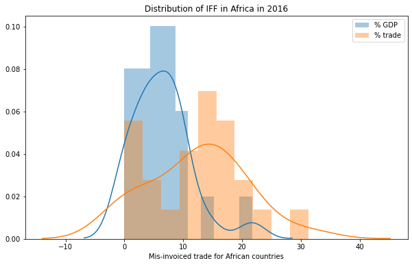
Mean outflow as proportion of GDP: 0.06371070220761896
Mean outflow as proportion of trade 0.006736362224603777
Those countries that experience disproportionately high outflows can be considered as “conduits” on which we can perform the network analysis.
We can use the figure above to inform our choice of thresholds for the proportion of IFF relative to GDP and trade, respectively, above which countries are considered conduits. Those thresholds are assigned to the variables thresh_GDP and thresh_trade, respectively.
thresh_GDP = 0.1
thresh_trade = 0.17
conduits_GDP = IFF_Year.query('Tot_IFF_hi_GDP >= @thresh_GDP').set_index('reporter.ISO')
conduits_trade = IFF_Year.query('Tot_IFF_hi_trade >= @thresh_trade').set_index('reporter.ISO')
The conduit countries respective to GDP are the Seychelles, where illicit outflows represented 22% of GDP in 2016, followed by Mozambique, Mali, and Tunisia.
| reporter | year | Tot_IFF_hi_GDP | GDP | |
|---|---|---|---|---|
| reporter.ISO | ||||
| MLI | Mali | 2016 | 0.102023 | 1.401079e+10 |
| MOZ | Mozambique | 2016 | 0.141781 | 1.098136e+10 |
| SYC | Seychelles | 2016 | 0.216881 | 1.427525e+09 |
| TUN | Tunisia | 2016 | 0.100490 | 4.180838e+10 |
The countries which experienced the highest level of mis-invoicing relative to their trading activity in 2016 were Burundi, where up to 31% of trade was illicit, followed by Uganda and Mali. Mali and Mozambique are conduit countries both when considering outflows relative to GDP and relative to trade openness.
| reporter | year | Tot_IFF_hi_trade | Total_value | |
|---|---|---|---|---|
| reporter.ISO | ||||
| DZA | Algeria | 2016 | 0.175611 | 77082785056 |
| BDI | Burundi | 2016 | 0.312707 | 754378325 |
| MLI | Mali | 2016 | 0.210566 | 6788467564 |
| MOZ | Mozambique | 2016 | 0.180047 | 8647421818 |
| NGA | Nigeria | 2016 | 0.179441 | 68077346474 |
| STP | São Tomé and Príncipe | 2016 | 0.204593 | 149825956 |
| UGA | Uganda | 2016 | 0.233074 | 7802352503 |
Finally, in addition to restricting our graph to certain conduit countries where the capital flows out of, we should also threshold on the partner countries to which the mis-invoiced capital flows in to. The figure below illustrates the distribution of illicit inflows as a proportion of their GDP for each partner country included in our bilateral flow data. That is, the weight on the edge from reporter \(i\) to partner \(j\) is relative to each partner \(j\)’s GDP in the chosen year. The magnitudes are smaller than the previous figure which considers the distribution of illicit outflows for each reporter \(i\) aggregated over all partners \(j\).
# Import data where value of illicit flow is standardized for partners
IFF_std = pd.read_csv('Data/GER_Orig_Dest_Year_std.csv')
IFF_std = IFF_std.query('year == "2016"')
# Merge in with flow data
flow_data = pd.merge(left=create_graph_data('2016', threshold_var='GDP'),
right=IFF_std[['reporter.ISO', 'partner.ISO', 'pImp_IFF_hi_GDP']],
on=['reporter.ISO', 'partner.ISO'])
# Plot distribution of IFF in partner countries
sns.distplot(flow_data['pImp_IFF_hi_GDP'], kde=True);
plt.title('Distribution of IFF in partner countries in 2016 (dyad-level)')
plt.xlabel('Mis-invoiced trade as proportion of GDP in partner countries');
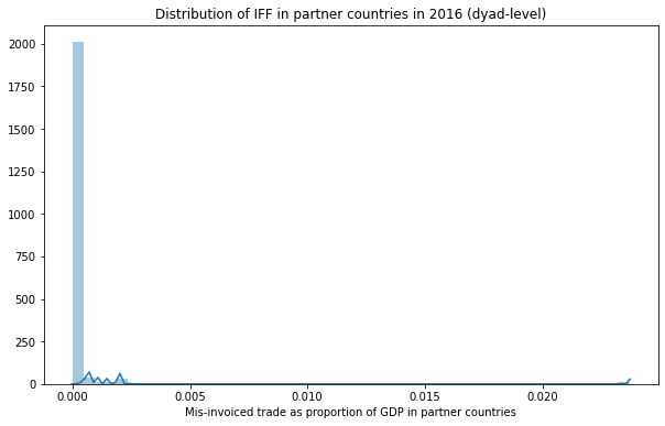
The distribution of outflows is heavily right-skewed, where the yearly outflow in 2016 from a single country to their partner resulted in an inflow to said partner which sometimes represented up to 2% of their GDP.
The helper function threshold_partner_IFF() thus helps us further threshold our bilateral flow data from the partner country perspective. By default, it restricts those bilateral flows to transactions where the inflow to the partner represented at least 0.01% of their GDP.
def threshold_partner_IFF(flow_data, year='2016', partner_threshold=0.0001):
"""
Filters bilateral flow data-set to minimum level of illicit flow relative to partner GDP.
flow_data: as Pandas dataframe, name of data-set which contains bilateral flow data
(in wide format)
year: as string, specify which year to use for the network analysis (between 2000-2016)
partner_threshold: as numeric, specify the cut-off for the minimum proportion of partner
GDP that a bilateral flow must represent in order to be included
"""
IFF_std = pd.read_csv('Data/GER_Orig_Dest_Year_std.csv')
IFF_std = IFF_std.query('year == @year')
flow_data = pd.merge(left=flow_data,
right=IFF_std[['reporter.ISO', 'partner.ISO', 'pImp_IFF_hi_GDP']],
on=['reporter.ISO', 'partner.ISO'])
flow_data = flow_data.query('pImp_IFF_hi_GDP >= @partner_threshold')
return flow_data
Let’s now create the directed graph data for countries which are conduits for illicit outflows relative to GDP and relative to trade value, respectively, and further restrict the data to edges where the mis-invoiced trade represents at least 0.01% of partner GDP.
Directed graph for GDP
Let’s create a directed graph for the flow data restricted to the top origins of illicit outflows relative to GDP, and applying the standard thresholding described above.
# Graph data for conduits relative to GDP
flow_data_GDP = create_graph_data('2016', threshold_var='GDP')
flow_data_GDP = threshold_partner_IFF(flow_data_GDP)
# Create directed graph
graph = nx.from_pandas_edgelist(flow_data_GDP,
'reporter.ISO',
'partner.ISO',
'Imp_IFF_hi',
create_using = nx.DiGraph())
This graph contains 33 vertices (or nodes) and 36 edges.
# Check the number of nodes and edges in the graph
len(graph.nodes()), len(graph.edges())
(33, 36)
# Print some of the edges in the network
list(graph.edges(data=True))[0:10]
[('MLI', 'GHA', {'Imp_IFF_hi': 8081515.07373014}),
('MLI', 'SEN', {'Imp_IFF_hi': 449650318.36780304}),
('MLI', 'ZAF', {'Imp_IFF_hi': 66862258.2240592}),
('MLI', 'TGO', {'Imp_IFF_hi': 9367585.98900624}),
('MLI', 'MRT', {'Imp_IFF_hi': 1267279.60791437}),
('MOZ', 'NAM', {'Imp_IFF_hi': 1165110.23690534}),
('MOZ', 'NLD', {'Imp_IFF_hi': 128444043.062896}),
('MOZ', 'PRT', {'Imp_IFF_hi': 121508025.10009299}),
('MOZ', 'SGP', {'Imp_IFF_hi': 466068356.77873796}),
('MOZ', 'ZAF', {'Imp_IFF_hi': 246975704.837192})]
In a directed graph, the degree of a node is the sum of its indegree (the number of edges going in to the node) and its outdegree (the number of edges going out of the node). In this case, the GDP conduit countries of Mali, Mozambique, Seychelles, and Tunisia will have a degree of a least 1 (corresponding to the outdegree of at least one edge going out).
# Get the degree of the nodes
graph.degree
DiDegreeView({'MLI': 5, 'GHA': 1, 'SEN': 1, 'ZAF': 3, 'TGO': 1, 'MOZ': 7, 'NAM': 1, 'NLD': 2, 'PRT': 2, 'SGP': 2, 'SYC': 3, 'MUS': 2, 'TUN': 21, 'DZA': 1, 'AZE': 1, 'BEL': 1, 'BGR': 1, 'HRV': 1, 'DNK': 1, 'EGY': 1, 'FRA': 1, 'HUN': 1, 'ITA': 1, 'JOR': 1, 'MYS': 1, 'MRT': 2, 'PRY': 1, 'RUS': 1, 'SVK': 1, 'SVN': 1, 'TUR': 1, 'UKR': 1, 'FIN': 1})
The function below achieves the following:
color the country nodes according to their GDP per capita;
color the edges according to the size of the logged illicit flow;
size the nodes proportionately to their degree (for use in the map case);
only label nodes with an outdegree of at least 1, that is, only the origin conduit countries selected by the thresholding above will have labels (for use in the map case).
def set_graph_attributes(graph):
"""
Sets node attributes and create auxiliary variables to be used in graph visualization.
Returns:
col: list of values to color nodes according to (node GDP per capita)
edge_col: array of values to color edges according to (logged flow between nodes)
sizes: list of values to size nodes (proportional to degree)
labels: dict of node labels (where a node is labelled if outdegree is at least 1)
"""
# Create dictionary of GDP per capita for each country
GDP_attr = covariates.loc[:, ['gdp-pc']]
GDP_attr = GDP_attr.to_dict('index')
# Set GDP per capita as a node attribute
nx.set_node_attributes(graph, GDP_attr)
# Create list of colors for nodes in the graph
col = [nx.get_node_attributes(graph, 'gdp-pc')[n] for n in graph.nodes]
# Create list of colors for edges in the graph
edge_col = [nx.get_edge_attributes(graph, 'Imp_IFF_hi')[e] for e in graph.edges]
edge_col = np.log(edge_col)
# Extract outdegree (the number of edges coming out of nodes) and degree
outdeg = graph.out_degree
deg = graph.degree
# Size of nodes will be proportional to their degree
sizes = [10 * deg[c] for c in graph.nodes]
# Label the countries if their outdegree is at least 1, i.e. if they are the reporting African countries
labels = {c: c if outdeg[c] >= 1 else ''
for c in graph.nodes}
return col, edge_col, outdeg, deg, sizes, labels
# Generate graph attributes and auxiliary variables
col, edge_col, outdeg, deg, sizes, labels = set_graph_attributes(graph)
We can now draw the network of illicit flows from the top 4 origins of illicit outflows with respect to GDP.
# Draw directed graph and color nodes by GDP per capita
plt.figure(figsize = (10,8))
pos = nx.spring_layout(graph)
nodes = nx.draw_networkx_nodes(graph, pos,
node_color=col, cmap=plt.cm.spring_r)
edges = nx.draw_networkx_edges(graph, pos,
edge_color=edge_col,
edge_cmap=plt.cm.get_cmap('RdPu'))
thous_fmt = FuncFormatter(lambda x, p: format(int(x), ','))
nx.draw_networkx_labels(graph, pos, font_size=10)
clb = plt.colorbar(nodes, format=thous_fmt)
clb.ax.set_title('GDP per capita');
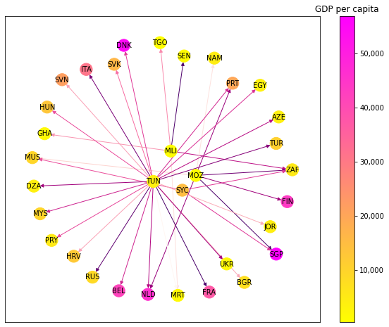
While the network visualization above is informative, the position of the nodes is generated using a force-directed algorithm. However, the nodes have an intuitive positioning in cartographical coordinates. Therefore, I exploit this implicit positioning and project the nodes above in a space spanned by longitude and latitude.
Thus, let us extract the longitude and latitude of the countries in order to position the nodes on the map.
# Create dictionary of longitude and latitude for countries
geo_pos = {country: (v['Longitude'], v['Latitude'])
for country, v in
crosswalk.drop_duplicates('ISO3166.3').set_index('ISO3166.3').to_dict('index').items()
}
list(geo_pos.items())[0:10]
[('ABW', (-69.98267711, 12.52088038)),
('AFG', (66.00473366, 33.83523073)),
('AGO', (17.53736768, -12.29336054)),
('AIA', (-63.06498927, 18.2239595)),
('ALA', (19.95328768, 60.21488688)),
('ALB', (20.04983396, 41.14244989)),
('AND', (1.56054378, 42.54229102)),
('ANT', (nan, nan)),
('ARE', (54.300167099999996, 23.90528188)),
('ARG', (-65.17980692, -35.3813488))]
# Map projection
crs = ccrs.PlateCarree()
fig, ax = plt.subplots(1, 1, figsize=(20, 8), subplot_kw=dict(projection=crs))
ax.coastlines(color='lightgray')
ax.add_feature(cfeature.LAND, facecolor='lightgray')
ax.add_feature(cfeature.BORDERS, edgecolor='white')
# Uncomment for the map to span the whole world
# ax.set_extent([-160, 180, -60, 90], crs=ccrs.PlateCarree())
# Overlay network graph
nx.draw_networkx(graph, ax=ax,
pos=geo_pos,
font_size=14,
alpha=0.7,
node_color=col, cmap=plt.cm.spring_r,
edge_color=edge_col, edge_cmap=plt.cm.get_cmap('RdPu'),
node_size=sizes,
labels=labels)
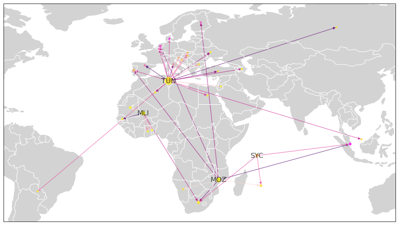
Directed graph for trade
Now, let’s create a directed graph for the flow data restricted to the top origins of illicit outflows relative to trade value, and applying the standard thresholding described above.
# Graph data for conduits relative to trade
flow_data_trade = create_graph_data('2016', threshold_var='trade')
flow_data_trade = threshold_partner_IFF(flow_data_trade)
# Create directed graph
graph = nx.from_pandas_edgelist(flow_data_trade,
'reporter.ISO',
'partner.ISO',
'Imp_IFF_hi',
create_using = nx.DiGraph())
This graph contains 70 vertices and 99 edges.
# Check the number of nodes and edges in the graph
len(graph.nodes()), len(graph.edges())
(70, 99)
# Generate graph attributes and auxiliary variables
col, edge_col, outdeg, deg, sizes, labels = set_graph_attributes(graph)
The network of illicit flows from the top origins of illicit outflows relative to trade value is displayed below.
# Draw directed graph and color nodes by GDP per capita
plt.figure(figsize = (10,8))
pos = nx.spring_layout(graph)
nodes = nx.draw_networkx_nodes(graph, pos,
node_color=col, cmap=plt.cm.spring_r)
edges = nx.draw_networkx_edges(graph, pos,
edge_color=edge_col,
edge_cmap=plt.cm.get_cmap('RdPu'))
thous_fmt = FuncFormatter(lambda x, p: format(int(x), ','))
nx.draw_networkx_labels(graph, pos, font_size=10)
clb = plt.colorbar(nodes, format=thous_fmt)
clb.ax.set_title('GDP per capita');
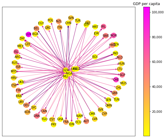
Finally, the figure below visualizes the directed graph on a map.
# Map projection
crs = ccrs.PlateCarree()
fig, ax = plt.subplots(1, 1, figsize=(20, 8), subplot_kw=dict(projection=crs))
ax.coastlines(color='lightgray')
ax.add_feature(cfeature.LAND, facecolor='lightgray')
ax.add_feature(cfeature.BORDERS, edgecolor='white')
# Uncomment for the map to span the whole world
# ax.set_extent([-160, 180, -60, 90], crs=ccrs.PlateCarree())
# Overlay network graph
nx.draw_networkx(graph, ax=ax,
pos=geo_pos,
font_size=14,
alpha=0.7,
node_color=col, cmap=plt.cm.spring_r,
edge_color=edge_col, edge_cmap=plt.cm.get_cmap('RdPu'),
node_size=sizes,
labels=labels)
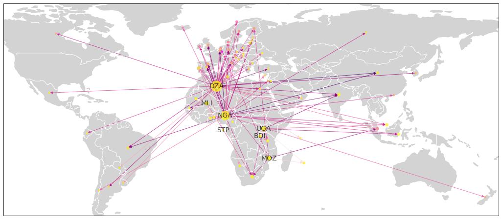
Evolution of the network during 2000-2016
The gif below displays the evolution of the network of illicit trade originating from Africa during 2000-2016 (i.e. the period for which we have data). The darkness of the edges (reflecting the logged dollar value of illicit trade) increased markedly during 2008-2009, perhaps reflecting the commodity supercycle at the time. If prices of internationally traded commodities increased, then it stands to reason that the dollar value of mis-invoiced trade increased as well.
Europe is a destination hub for illicit outflows originating in Africa. The size of the nodes is proportional to their degree. The size of European nodes increased during 2008-2012 and decreased in 2015-2016.
# Create network maps of illicit flows for 2000-2016
for y in range(2000, 2017, 1):
# Entire network of illicit flows in 2016
flow_data_whole = create_graph_data(str(y), threshold=False, flow_threshold=1000000)
# Create directed graph
graph = nx.from_pandas_edgelist(flow_data_whole,
'reporter.ISO',
'partner.ISO',
'Imp_IFF_hi',
create_using = nx.DiGraph())
# Set map attributes
col, edge_col, outdeg, deg, sizes, labels = set_graph_attributes(graph)
# Map projection
crs = ccrs.PlateCarree()
fig, ax = plt.subplots(1, 1, figsize=(20, 8), subplot_kw=dict(projection=crs))
ax.coastlines(color='lightgray')
ax.add_feature(cfeature.LAND, facecolor='lightgray')
ax.add_feature(cfeature.BORDERS, edgecolor='white')
# Uncomment for the map to span the whole world
ax.set_extent([-160, 180, -60, 90], crs=ccrs.PlateCarree())
# Overlay network graph
nx.draw_networkx(graph, ax=ax,
pos=geo_pos,
font_size=14,
alpha=0.7,
node_color=col, cmap=plt.cm.spring_r,
edge_color=edge_col, edge_cmap=plt.cm.get_cmap('RdPu'),
node_size=sizes,
labels=labels);
fig.suptitle('Network of illicit outflows originating in Africa in ' + str(y), fontsize=20)
plt.savefig('Images/Network_Maps/network_map_' + str(y) + '.png')
plt.clf();
# Create gif from network map images
filenames = ['Images/Network_Maps/network_map_' + str(y) + '.png' for y in range(2000, 2017, 1)]
images = []
for filename in filenames:
images.append(imageio.imread(filename))
imageio.mimsave('Images/Network_Maps/Maps.gif', images, duration=2)

Conclusion
This project has utilized the newest estimates of trade mis-invoicing of the United Nations Economic Commission for Africa (http://doi.org/10.5281/zenodo.3610558). The data contains estimates of the dollar value of illicit trade in both imports and exports for all reporting jurisdictions in the UN COMTRADE database, for 21 commodity sectors during the period 2000-2016.
Following the establishment of the High Level Panel on Illicit Financial Flows from Africa in 2015, the scale and severity of the problem has been well-recognized by policy-makers and NGOs. The next steps now are to move beyond scale estimates and to start understanding the nature, mechanisms, and directions of illicit trade on the continent. This project takes the first steps towards that goal.
I have utilized unsupervised machine learning techniques such as dimension reduction, clustering, and network analysis to extract meaningful insights from the data. Given that the feature space is large, especially when analyzing the data in its dyadic form, dimension reduction techniques are necessary to project the data in a lower-dimensional space.
Following that, I explored some clustering techniques to ascertain whether they were able to recover some of the ground truth labels of the observations such as regional groups or income classification. Cluster validation will require further work.
Finally, I exploited the bilateral nature of the data and perfomed a preliminary network analysis for illicit trade originating from African countries. Given the methodology used to estimate mis-invoicing, an edge would be created between a reporter-partner pair for any discrepancy in mirrored trade statistics. Therefore, it is necessary to apply thresholding before conducting network analysis. Further work will need to examine network statistics such as centrality measures in order to yield further insights.
Policy recommendations
Target 16.4 of the SDGs: “By 2030, significantly reduce illicit financial and arms flows, strengthen the recovery and return of stolen assets and combat all forms of organized crime”
Estimates of the magnitude and severity of the problem have shed a spotlight on the need to combat illicit financial flows
Deeper understanding of the origins and destinations is now crucial to guiding targeted interventions to combat illicit flows
Strong subregional effects are apparent in illicit trade within the continent. Initiatives to combat illicit flows could be anchored within the Regional Economic Communities of the African Union, such as ECOWAS.
Next steps
I plan to take this project further. Notably, I plan to conduct analysis on the most disaggregated view of the data, that is, for a reporter-partner-year-commodity tuple. By filtering by commodity sector, I will be able to identify the relevant sinks and sources.
Moreover, I am currently exploring spectral clustering. However, spectral clustering algorithms are currently implemented for undirected rather than directed graphs. There are several possible approaches to dealing with clustering on directed graphs. One of them includes a naive approach where direction is ignored, and where the graph is treated as an undirected network.
Finally, I am considering non-negative matrix factorization as an alternative form of dimension reduction.