Unsupervised learning on illicit trade data
Alice Lépissier
Bren School of Environmental Science and Management
Policy and media attention on illicit financial flows (IFF) has increased, with the recognition that Africa is a net creditor to the world.
 |
 |
|
| New York Times (2013) | Guardian (2015) | |
 |
 | |
| Guardian (2017) | Economist (2019) |
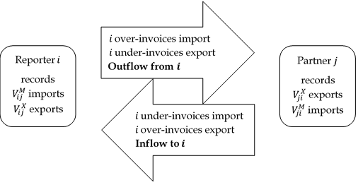
What is trade mis-invoicing?
- The deliberate mis-statement of price or quantity of internationally traded goods in invoices presented to customs
- Can occur at import or export
- Can result in an inflow or outflow of money
Motivations for trade mis-invoicing include:
- Evading tariffs
- Exploiting subsidy regimes
- Subverting forex and capital controls
- Hiding transfers of wealth
Mechanisms of mis-invoicing
Why does trade mis-invoicing matter?
- Outflows undermine the fiscal base and public spending
- Financing gap needed to meet the Sustainable Development Goals (SDGs)
- Combating trade mis-invoicing is crucial for the mobilization of domestic resources in the continent, and can catalyze sustainable development
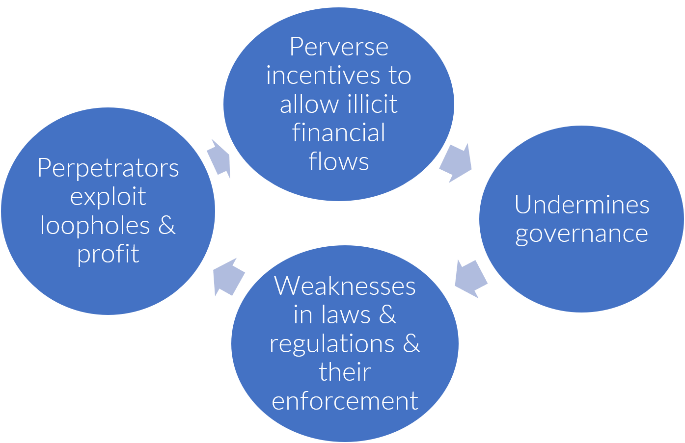 |
| Governance loop (credit: William Davis) |
Data source
- Trade mis-invoicing data-set of the United Nations Economic Commission for Africa
- Panel with $n=6,248,254$ of mis-invoiced trade between 179 reporting jurisdictions and 179 partner countries for years 2000-2016 and disaggregated commodities
- Citation: Lépissier, Alice, Davis, William, & Ibrahim, Gamal. (2019). Trade Mis-Invoicing Dataset (Version 1).

- The entire data-set
panel_results.Rdatawith ~6 million observations is available online. - The unit of observation is a reporter-partner-commodity-year tuple, where the data represent the illicit flow embedded in a transaction between a reporter $i$ and a partner $j$ for a commodity $c$ in year $t$.
- The full panel is ~2GB. This notebook works with smaller summary data-sets generated from the full panel. The code to generate these summary data-sets is available on the repository https://github.com/walice/Trade-IFF by running the script file
Compute IFF Estimates.R.
Methodology for calculating mis-invoiced trade
- We locate mis-invoicing in the discrepancies between reported trade flows and their mirrored statistics
- But not all observed discrepancies are due to illicit motives!
- Imports tend to be recorded on the basis of Cost of Insurance and Freight (CIF), while exports are recorded Free On Board (FOB)
Our approach
- Estimate the discrepancies between imports and mirror net exports as a function of both licit and illicit predictors
- Perform a harmonization procedure in order to generate a reconciled value that represents our best estimate of what the legitimate value of the trade should be on a FOB basis
- Calculate the IFF embedded in each transaction as the difference between the observed value and the reconciled value
- The panel can be aggregated over several dimensions, e.g. partner country, commodity, year. There are two methods to aggregate up the illicit flow:
- Net basis: simply add up all negative and positive values, so that inflows and outflows cancel each other out
- Gross Excluding Reversals (GER) basis: ignore all inflows, and sum up the positive values only across trading partners
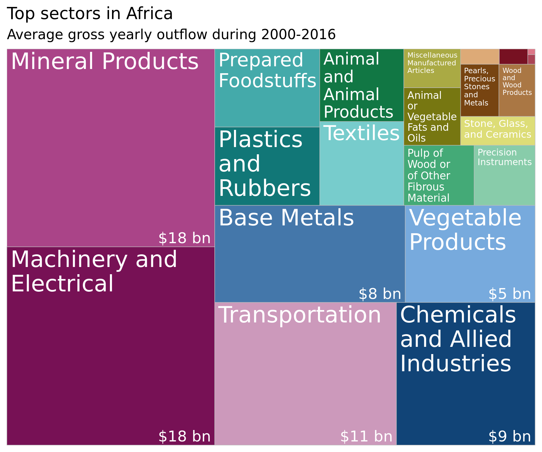
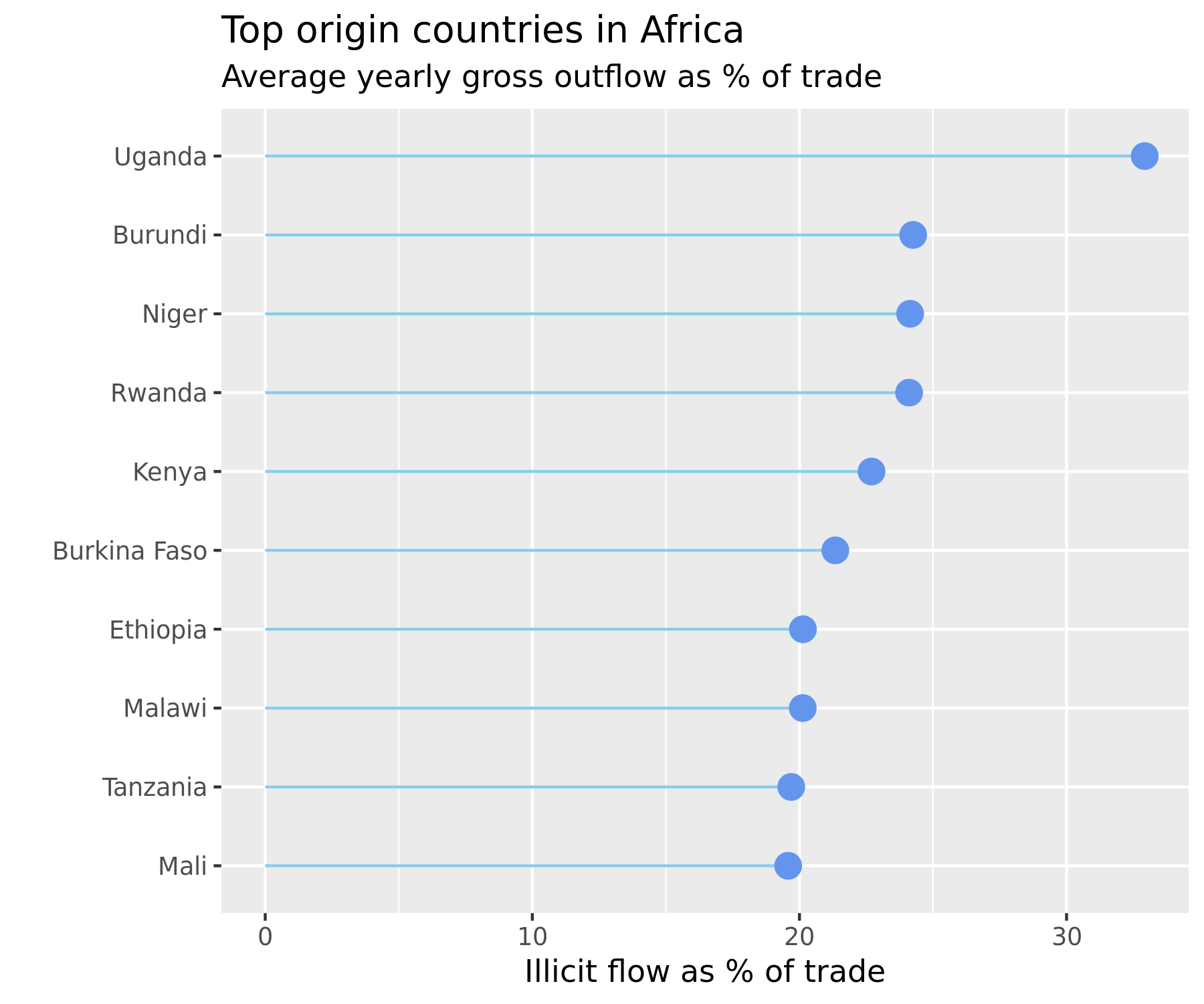
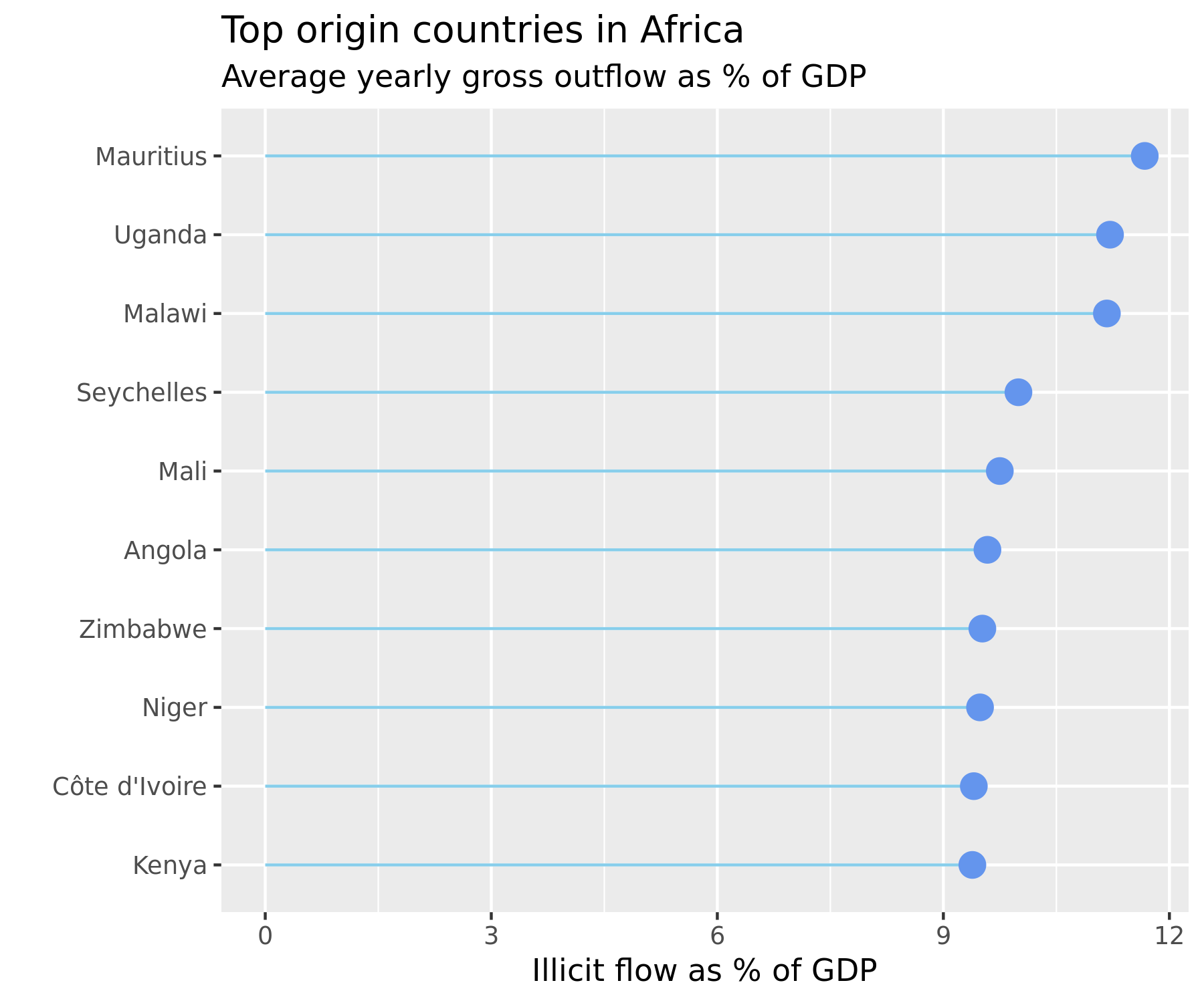
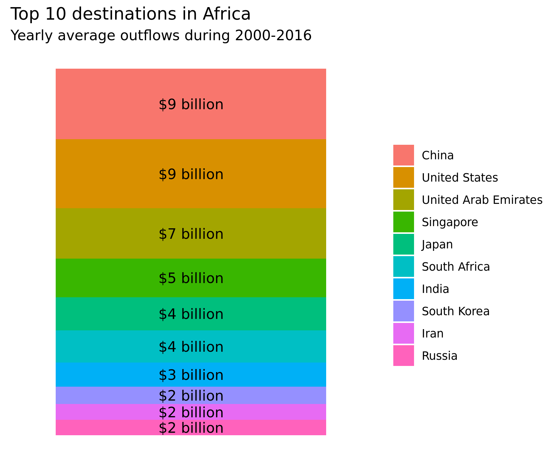
Zoom in on Africa
- During 2000-2016, the continent lost on average \$83 billion a year in gross illicit outflows
- Net cumulative flows during that period were \$362 billion
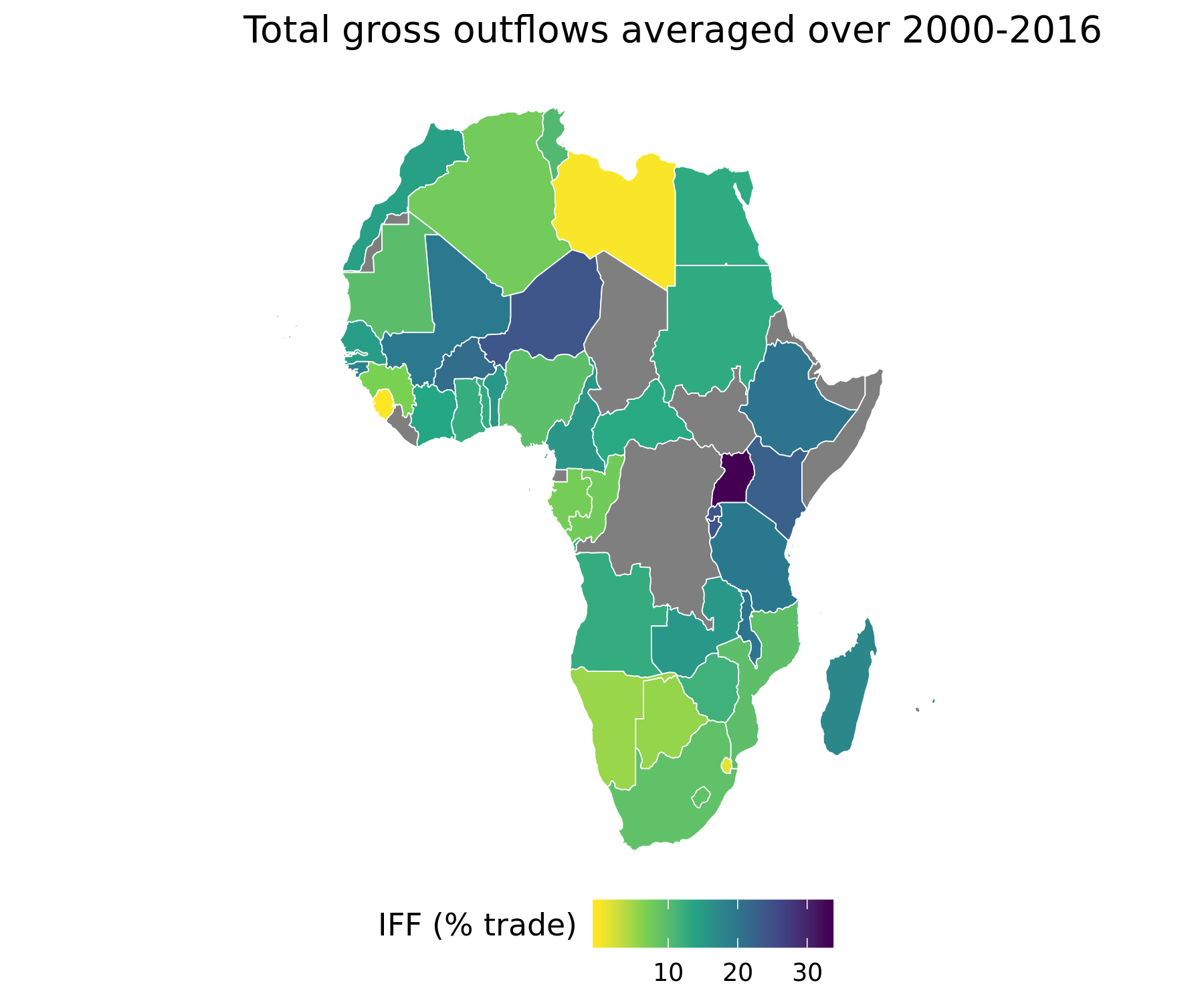 Source: generated by
 Data Visualization.R in https://github.com/walice/Trade-IFF
Goals
This project will apply the following techniques to the data:
- Dimension reduction using Principal Components Analysis (PCA)
- Clustering
- Graph analysis
Data wrangling
- Mis-invoiced trade for countries (aggregated data)
- View 1: unit of observation = reporter-year; features = sectors
- View 2: unit of observation = sector-year; features = reporters
- Bilateral matrix of mis-invoiced trade (dyadic data)
- Unit of observation = reporter-partner-year
Mis-invoiced trade for countries by sectors
# Extract mis-invoicing in imports
IFF_Sector_Imp = IFF_Sector[['section', 'Imp_IFF_hi']]
IFF_Sector_Imp
Mis-invoiced trade for dyads
# Extract mis-invoicing in imports
IFF_Dest_Imp = IFF_Dest[['partner.ISO', 'Imp_IFF_hi']]
IFF_Dest_Imp
Metadata for countries
crosswalk = pd.read_excel("Data/crosswalk.xlsx").rename(columns={'Country': 'country'})
crosswalk.head()
Auxiliary functions
def create_features(data, values, features, obs):
"""
Convert data-set in long format to wide and preserve information on year.
data: {IFF_Sector_Imp, IFF_Dest_Imp, IFF_Dest_AFR, ...}, as Pandas dataframe,
name of data-set from which to create feature space, must be in long format
values: {'Imp_IFF_hi', 'Exp_IFF_hi'}, as string, values that data-set will represent
features: {'reporter.ISO', 'section', 'partner.ISO'}, as string,
what to use as the feature space
obs: {'section', 'reporter.ISO'}, as string, what to use as the observation level
"""
features_data = data.pivot_table(values=values,
columns=features,
index=[obs, 'year'],
fill_value=0)
return features_data
def biplot_PCA(features_data, nPC=2, firstPC=1, secondPC=2, obs='reporter.ISO', show_loadings=False):
"""
Project the data in the 2-dimensional space spanned by 2 principal components
chosen by the user, along with a bi-plot of the top 3 loadings per PC, and color observations
by class label.
Args:
features_data: as Pandas dataframe, data-set of features
nPC: number of principal components
firstPC: integer denoting first principal component to plot in bi-plot
secondPC: integer denoting second principal component to plot in bi-plot
obs: string denoting index of class labels (in features_data)
show_loadings: Boolean indicating whether PCA loadings should be displayed
Returns:
plot (interactive)
pca_loadings (if show_loadings=True)
"""
# Run PCA (standardize data beforehand)
features_data_std = StandardScaler().fit_transform(features_data)
pca = PCA(n_components=nPC, random_state=234)
princ_comp = pca.fit_transform(features_data_std)
# Extract PCA loadings
cols = ['PC' + str(c+1) for c in np.arange(nPC)]
pca_loadings = pd.DataFrame(pca.components_.T,
columns=cols,
index=list(features_data.columns))
# Extract PCA scores
pca_scores = pd.DataFrame(princ_comp,
columns=cols)
pca_scores[obs] = features_data.reset_index()[obs].values.tolist()
pca_scores['year'] = features_data.reset_index()['year'].values.tolist()
score_PC1 = princ_comp[:,firstPC-1]
score_PC2 = princ_comp[:,secondPC-1]
# Generate plot data
if obs == 'reporter.ISO':
plot_data = pd.merge(pca_scores, obs_info, on=[obs, 'year'])
color_obs = 'reporter'
tooltip_obs = ['reporter', 'year', 'Income group (World Bank)', 'Country status (UN)']
else:
plot_data = pca_scores
color_obs = 'section'
tooltip_obs = ['section', 'year']
# Return chosen PCs to plot
PC1 = 'PC'+str(firstPC)
PC2 = 'PC'+str(secondPC)
# Extract top loadings (in absolute value)
# TO DO: use dict to iterate over
toploadings_PC1 = pca_loadings.apply(lambda x: abs(x)).sort_values(by=PC1).tail(3)[[PC1, PC2]]
toploadings_PC2 = pca_loadings.apply(lambda x: abs(x)).sort_values(by=PC2).tail(3)[[PC1, PC2]]
originsPC1 = pd.DataFrame({'index':toploadings_PC1.index.tolist(),
PC1: np.zeros(3),
PC2: np.zeros(3)})
originsPC2 = pd.DataFrame({'index':toploadings_PC2.index.tolist(),
PC1: np.zeros(3),
PC2: np.zeros(3)})
toploadings_PC1 = pd.concat([toploadings_PC1.reset_index(), originsPC1], axis=0)
toploadings_PC2 = pd.concat([toploadings_PC2.reset_index(), originsPC2], axis=0)
toploadings_PC1[PC1] = toploadings_PC1[PC1]*max(score_PC1)*1.5
toploadings_PC1[PC2] = toploadings_PC1[PC2]*max(score_PC2)*1.5
toploadings_PC2[PC1] = toploadings_PC2[PC1]*max(score_PC1)*1.5
toploadings_PC2[PC2] = toploadings_PC2[PC2]*max(score_PC2)*1.5
# Project top 3 loadings over the space spanned by 2 principal components
lines = alt.Chart().mark_line().encode()
for color, i, dataset in zip(['#440154FF', '#21908CFF'], [0,1], [toploadings_PC1, toploadings_PC2]):
lines[i] = alt.Chart(dataset).mark_line(color=color).encode(
x= PC1 +':Q',
y= PC2 +':Q',
detail='index'
).properties(
width=400,
height=400
)
# Add labels to the loadings
text=alt.Chart().mark_text().encode()
for color, i, dataset in zip(['#440154FF', '#21908CFF'], [0, 1], [toploadings_PC1[0:3], toploadings_PC2[0:3]]):
text[i] = alt.Chart(dataset).mark_text(
align='left',
baseline='bottom',
color=color
).encode(
x= PC1 +':Q',
y= PC2 +':Q',
text='index'
)
# Scatter plot colored by observation class label
points = alt.Chart(plot_data).mark_circle(size=60).encode(
x=alt.X(PC1, axis=alt.Axis(title='Principal Component ' + str(firstPC))),
y=alt.X(PC2, axis=alt.Axis(title='Principal Component ' + str(secondPC))),
color=alt.Color(color_obs, scale=alt.Scale(scheme='category20b'),
legend=alt.Legend(orient='right')),
tooltip=tooltip_obs
).interactive()
# Bind it all together
chart = (points + lines[0] + lines[1] + text[0] + text[1])
chart.display()
if show_loadings:
return pca_loadings
def scree_plot(features_data, show_explained_var=False):
"""
Create a cumulative scree splot and (optional) return the explained variance by each component.
features_data: as Pandas dataframe, the data-set on which to run PCA
show_explained_var: as Boolean, flag for whether to return explained variance
"""
features_data_std = StandardScaler().fit_transform(features_data)
pca = PCA(n_components=features_data_std.shape[1], random_state=234)
princ_comp = pca.fit_transform(features_data_std)
explained_var = pd.DataFrame({'PC': np.arange(1,features_data_std.shape[1]+1),
'var': pca.explained_variance_ratio_,
'cumvar': np.cumsum(pca.explained_variance_ratio_)})
# Adapted from https://altair-viz.github.io/gallery/multiline_tooltip.html
# Create a selection that chooses the nearest point & selects based on x-value
nearest = alt.selection(type='single', nearest=True, on='mouseover',
fields=['PC'], empty='none')
# The basic line
line = alt.Chart(explained_var).mark_line(interpolate='basis', color='#FDE725FF').encode(
alt.X('PC:Q',
scale=alt.Scale(domain=(1, len(explained_var))),
axis=alt.Axis(title='Principal Component')
),
alt.Y('cumvar:Q',
scale=alt.Scale(domain=(min(explained_var['cumvar']), 1)),
axis=alt.Axis(title='Cumulative Variance Explained')
),
)
# Transparent selectors across the chart. This is what tells us
# the x-value of the cursor
selectors = alt.Chart(explained_var).mark_point().encode(
x='PC:Q',
opacity=alt.value(0),
).add_selection(
nearest
)
# Draw points on the line, and highlight based on selection
points = line.mark_point().encode(
opacity=alt.condition(nearest, alt.value(1), alt.value(0))
)
# Draw text labels near the points, and highlight based on selection
text = line.mark_text(align='left', dx=5, dy=-5).encode(
text=alt.condition(nearest, 'cumvar:Q', alt.value(' '))
)
# Draw a rule at the location of the selection
rules = alt.Chart(explained_var).mark_rule(color='gray').encode(
x='PC:Q',
).transform_filter(
nearest
)
# Put the five layers into a chart and bind the data
out = alt.layer(
line, selectors, points, rules, text
).properties(
title='Cumulative scree plot',
width=500, height=300
)
out.display()
if show_explained_var:
return explained_var[['PC', 'var']]
PCA on feature space (for individual reporting countries)
Sector features
sector_features = create_features(IFF_Sector_Imp, 'Imp_IFF_hi',
features='section', obs='reporter.ISO')
sector_features
Biplots
biplot_PCA(sector_features, 10, 1, 2, obs='reporter.ISO', show_loadings=True)
 Source: generated by
 Data Visualization.R in https://github.com/walice/Trade-IFF
biplot_PCA(sector_features, 10, 5, 6, obs='reporter.ISO')
Explained variance
scree_plot(sector_features, show_explained_var=True)
Variance-stabilizing and normalizing transformations
# Plot distribution of illicit flow in each feature (i.e. sector)
fig, axes = joypy.joyplot(sector_features, colormap=plt.cm.viridis, figsize=(8,8),
title='Distribution of mis-invoicing across sectors');

sector_features_yeo = pd.DataFrame(sector_features_yeo,
index=sector_features.index,
columns=sector_features.columns)
fig, axes = joypy.joyplot(sector_features_yeo, colormap=plt.cm.viridis, figsize=(8,8),
title='Distribution of mis-invoicing across sectors (Yeo–Johnson transformation)');

biplot_PCA(sector_features_yeo, 10, 1, 2, obs='reporter.ISO')
Country features
country_features = create_features(IFF_Sector_Imp, 'Imp_IFF_hi',
features='reporter.ISO', obs='section')
country_features
Biplots
biplot_PCA(country_features, 10, 1, 2, obs='section', show_loadings=True)
 Source: generated by
 Data Visualization.R in https://github.com/walice/Trade-IFF)
 Source: generated by
 Data Visualization.R in https://github.com/walice/Trade-IFF)
Variance-stabilizing and normalizing transformations
biplot_PCA(country_features_log, 10, 1, 2, obs='section')
biplot_PCA(country_features_yeo, 10, 1, 2, obs='section')
PCA on bilateral trade matrix
partner_features = create_features(IFF_Dest_Imp, 'Imp_IFF_hi',
features='partner.ISO', obs='reporter.ISO')
partner_features
Biplots
biplot_PCA(partner_features, 10, 1, 2, show_loadings=True)
 Source: generated by
 Data Visualization.R in https://github.com/walice/Trade-IFF
Intra-African illicit financial flows
partner_features_AFR = create_features(IFF_Dest_Imp_AFR, 'Imp_IFF_hi',
features='partner.ISO', obs='reporter.ISO')
partner_features_AFR
biplot_PCA(partner_features_AFR, partner_features_AFR.shape[1], 1, 2)
Removing outliers
partner_features_AFR_noout = partner_features_AFR[~outlying]
biplot_PCA(partner_features_AFR_noout, 46, 1, 2)
Coloring by class label
biplot_PCA_classes(sector_features, 21, 1, 2, classes='Income group (World Bank)')
biplot_PCA_classes(partner_features, 46, 1, 2)
biplot_PCA_classes(partner_features_AFR_noout, 46, 1, 2)
Clustering
Agglomerative clustering
# Perform agglomerative clustering
from sklearn.cluster import AgglomerativeClustering
clustering = AgglomerativeClustering(n_clusters=5, linkage='ward').fit(X)
plt.scatter(X[:, 0], X[:, 1], c=clustering.labels_);
plt.title('Agglomerative clustering using Ward linkage');

Hierarchical clustering and corresponding heatmap
# Plot heatmap and corresponding dendograms
g = sns.clustermap(data_scaled,
method='ward',
cmap='bone_r',
row_colors=region_color,
);
g.fig.suptitle('Hierarchical clustering with Ward linkage', y=1);

Network analysis
def create_graph_data(year='2016', threshold=True, threshold_var='GDP', flow_threshold=10000):
"""
Returns data-set to be used to generate a directed graph.
year: as string, specify which year to use for the network analysis (between 2000-2016)
threshold: as boolean, indicate whether to restrict reporting countries to conduits
threshold_var: as string, indicate which variable to use when determining which
reporting countries are conduits ('GDP' or 'trade')
flow_threshold: as numeric, specify the cut-off under which to ignore the dollar values
of mis-invoiced imports
"""
flow_data = IFF_Dest.reset_index().query('year == @year')
flow_data = flow_data.loc[flow_data['Imp_IFF_hi'].notnull(), :]
flow_data = flow_data.query('Imp_IFF_hi >= @flow_threshold')
if threshold:
conduits = 'conduits_' + threshold_var
flow_data = flow_data[flow_data['reporter.ISO'].isin(eval(conduits).index)]
return flow_data
Thresholding
# Import data on mis-invoiced trade aggregated by destination and sector for each African country
IFF_Year = pd.read_csv('Data/GER_Orig_Year_Africa.csv')
# Restrict data to 2016 as an illustrative example
IFF_Year = IFF_Year.query('year == "2016"')
# Plot distribution of proportional mis-invoiced imports for each African country
sns.distplot(IFF_Year['Tot_IFF_hi_GDP'].apply(lambda x: x*100),
kde=True, label='% GDP', bins=10);
sns.distplot(IFF_Year['Tot_IFF_hi_trade'].apply(lambda x: x*100),
kde=True, label='% trade', bins=10);
plt.legend()
plt.title('Distribution of IFF in Africa in 2016')
plt.xlabel('Mis-invoiced trade for African countries');

print('Mean outflow as proportion of GDP:',IFF_Year['Tot_IFF_hi_GDP'].mean(),
'\nMean outflow as proportion of trade', IFF_Year['Tot_IFF_hi_trade'].var())
thresh_GDP = 0.1
thresh_trade = 0.17
conduits_GDP = IFF_Year.query('Tot_IFF_hi_GDP >= @thresh_GDP').set_index('reporter.ISO')
conduits_trade = IFF_Year.query('Tot_IFF_hi_trade >= @thresh_trade').set_index('reporter.ISO')
conduits_GDP[['reporter', 'year', 'Tot_IFF_hi_GDP', 'GDP']]
conduits_trade[['reporter', 'year', 'Tot_IFF_hi_trade', 'Total_value']]
# Import data where value of illicit flow is standardized for partners
IFF_std = pd.read_csv('Data/GER_Orig_Dest_Year_std.csv')
IFF_std = IFF_std.query('year == "2016"')
# Merge in with flow data
flow_data = pd.merge(left=create_graph_data('2016', threshold_var='GDP'),
right=IFF_std[['reporter.ISO', 'partner.ISO', 'pImp_IFF_hi_GDP']],
on=['reporter.ISO', 'partner.ISO'])
# Plot distribution of IFF in partner countries
sns.distplot(flow_data['pImp_IFF_hi_GDP'], kde=True);
plt.title('Distribution of IFF in partner countries in 2016 (dyad-level)')
plt.xlabel('Mis-invoiced trade as proportion of GDP in partner countries');

def threshold_partner_IFF(flow_data, year='2016', partner_threshold=0.0001):
"""
Filters bilateral flow data-set to minimum level of illicit flow relative to partner GDP.
flow_data: as Pandas dataframe, name of data-set which contains bilateral flow data
(in wide format)
year: as string, specify which year to use for the network analysis (between 2000-2016)
partner_threshold: as numeric, specify the cut-off for the minimum proportion of partner
GDP that a bilateral flow must represent in order to be included
"""
IFF_std = pd.read_csv('Data/GER_Orig_Dest_Year_std.csv')
IFF_std = IFF_std.query('year == @year')
flow_data = pd.merge(left=flow_data,
right=IFF_std[['reporter.ISO', 'partner.ISO', 'pImp_IFF_hi_GDP']],
on=['reporter.ISO', 'partner.ISO'])
flow_data = flow_data.query('pImp_IFF_hi_GDP >= @partner_threshold')
return flow_data
Directed graph for GDP
# Graph data for conduits relative to GDP
flow_data_GDP = create_graph_data('2016', threshold_var='GDP')
flow_data_GDP = threshold_partner_IFF(flow_data_GDP)
# Create directed graph
graph = nx.from_pandas_edgelist(flow_data_GDP,
'reporter.ISO',
'partner.ISO',
'Imp_IFF_hi',
create_using = nx.DiGraph())
def set_graph_attributes(graph):
"""
Sets node attributes and create auxiliary variables to be used in graph visualization.
Returns:
col: list of values to color nodes according to (node GDP per capita)
edge_col: array of values to color edges according to (logged flow between nodes)
sizes: list of values to size nodes (proportional to degree)
labels: dict of node labels (where a node is labelled if outdegree is at least 1)
"""
# Create dictionary of GDP per capita for each country
GDP_attr = covariates.loc[:, ['gdp-pc']]
GDP_attr = GDP_attr.to_dict('index')
# Set GDP per capita as a node attribute
nx.set_node_attributes(graph, GDP_attr)
# Create list of colors for nodes in the graph
col = [nx.get_node_attributes(graph, 'gdp-pc')[n] for n in graph.nodes]
# Create list of colors for edges in the graph
edge_col = [nx.get_edge_attributes(graph, 'Imp_IFF_hi')[e] for e in graph.edges]
edge_col = np.log(edge_col)
# Extract outdegree (the number of edges coming out of nodes) and degree
outdeg = graph.out_degree
deg = graph.degree
# Size of nodes will be proportional to their degree
sizes = [10 * deg[c] for c in graph.nodes]
# Label the countries if their outdegree is at least 1, i.e. if they are the reporting African countries
labels = {c: c if outdeg[c] >= 1 else ''
for c in graph.nodes}
return col, edge_col, outdeg, deg, sizes, labels
# Generate graph attributes and auxiliary variables
col, edge_col, outdeg, deg, sizes, labels = set_graph_attributes(graph)
# Draw directed graph and color nodes by GDP per capita
plt.figure(figsize = (10,8))
pos = nx.spring_layout(graph)
nodes = nx.draw_networkx_nodes(graph, pos,
node_color=col, cmap=plt.cm.spring_r)
edges = nx.draw_networkx_edges(graph, pos,
edge_color=edge_col,
edge_cmap=plt.cm.get_cmap('RdPu'))
thous_fmt = FuncFormatter(lambda x, p: format(int(x), ','))
nx.draw_networkx_labels(graph, pos, font_size=10)
clb = plt.colorbar(nodes, format=thous_fmt)
clb.ax.set_title('GDP per capita');

# Create dictionary of longitude and latitude for countries
geo_pos = {country: (v['Longitude'], v['Latitude'])
for country, v in
crosswalk.drop_duplicates('ISO3166.3').set_index('ISO3166.3').to_dict('index').items()
}
list(geo_pos.items())[0:10]
# Map projection
crs = ccrs.PlateCarree()
fig, ax = plt.subplots(1, 1, figsize=(20, 8), subplot_kw=dict(projection=crs))
ax.coastlines(color='lightgray')
ax.add_feature(cfeature.LAND, facecolor='lightgray')
ax.add_feature(cfeature.BORDERS, edgecolor='white')
# Uncomment for the map to span the whole world
# ax.set_extent([-160, 180, -60, 90], crs=ccrs.PlateCarree())
# Overlay network graph
nx.draw_networkx(graph, ax=ax,
pos=geo_pos,
font_size=14,
alpha=0.7,
node_color=col, cmap=plt.cm.spring_r,
edge_color=edge_col, edge_cmap=plt.cm.get_cmap('RdPu'),
node_size=sizes,
labels=labels)

Directed graph for trade
# Graph data for conduits relative to trade
flow_data_trade = create_graph_data('2016', threshold_var='trade')
flow_data_trade = threshold_partner_IFF(flow_data_trade)
# Create directed graph
graph = nx.from_pandas_edgelist(flow_data_trade,
'reporter.ISO',
'partner.ISO',
'Imp_IFF_hi',
create_using = nx.DiGraph())
# Generate graph attributes and auxiliary variables
col, edge_col, outdeg, deg, sizes, labels = set_graph_attributes(graph)
# Draw directed graph and color nodes by GDP per capita
plt.figure(figsize = (10,8))
pos = nx.spring_layout(graph)
nodes = nx.draw_networkx_nodes(graph, pos,
node_color=col, cmap=plt.cm.spring_r)
edges = nx.draw_networkx_edges(graph, pos,
edge_color=edge_col,
edge_cmap=plt.cm.get_cmap('RdPu'))
thous_fmt = FuncFormatter(lambda x, p: format(int(x), ','))
nx.draw_networkx_labels(graph, pos, font_size=10)
clb = plt.colorbar(nodes, format=thous_fmt)
clb.ax.set_title('GDP per capita');

# Map projection
crs = ccrs.PlateCarree()
fig, ax = plt.subplots(1, 1, figsize=(20, 8), subplot_kw=dict(projection=crs))
ax.coastlines(color='lightgray')
ax.add_feature(cfeature.LAND, facecolor='lightgray')
ax.add_feature(cfeature.BORDERS, edgecolor='white')
# Uncomment for the map to span the whole world
# ax.set_extent([-160, 180, -60, 90], crs=ccrs.PlateCarree())
# Overlay network graph
nx.draw_networkx(graph, ax=ax,
pos=geo_pos,
font_size=14,
alpha=0.7,
node_color=col, cmap=plt.cm.spring_r,
edge_color=edge_col, edge_cmap=plt.cm.get_cmap('RdPu'),
node_size=sizes,
labels=labels)

Evolution of the network during 2000-2016

Conclusion
Policy recommendations
- Target 16.4 of the SDGs: "By 2030, significantly reduce illicit financial and arms flows, strengthen the recovery and return of stolen assets and combat all forms of organized crime"
- Estimates of the magnitude and severity of the problem have shed a spotlight on the need to combat illicit financial flows
- Deeper understanding of the origins and destinations is now crucial to guiding targeted interventions to combat illicit flows
- Strong subregional effects are apparent in illicit trade within the continent. Initiatives to combat illicit flows could be anchored within the Regional Economic Communities of the African Union, such as ECOWAS.
Next steps
I plan to take this project further. Notably, I plan to conduct analysis on the most disaggregated view of the data, that is, for a reporter-partner-year-commodity tuple. By filtering by commodity sector, I will be able to identify the relevant sinks and sources.
Moreover, I am currently exploring spectral clustering. However, spectral clustering algorithms are currently implemented for undirected rather than directed graphs. There are several possible approaches to dealing with clustering on directed graphs. One of them includes a naive approach where direction is ignored, and where the graph is treated as an undirected network.
Finally, I am considering non-negative matrix factorization as an alternative form of dimension reduction.